This post is an addendum to the excellent paper Scalable Reward Distribution on the Ethereum Blockchain by Batog et al.¹ The outlined algorithm describes a pull-based approach to distributing rewards proportionally in a staking pool. In other words, instead of pushing rewards to each stakeholder in a for-loop with $O(n)$ complexity, a mathematical trick enables keeping account of the rewards with $O(1)$ complexity and distributing only when the stakeholders decide to pull them. This allows the distribution of things like rewards, dividends, Universal Basic Income, etc. with minimal resources and huge scalability.

The paper by Bogdan et al. assumes a model where stake size doesn’t change once it is deposited, presumably to explain the concept in the simplest way possible. After the deposit, a stakeholder can wait to collect rewards and then withdraw both the deposit and the accumulated rewards. This would rarely be the case in real applications, as participants would want to increase or decrease their stakes between reward distributions. To make this possible, we need to make modifications to the original formulation and algorithm. Note that the algorithm given below is already implemented in PoWH3D.

In the paper, the a $\text{reward}_t$ is distributed to a participant $j$ with an associated $\text{stake}_j$ as

\[\text{reward}_{j,t} = \text{stake}_{j} \frac{\text{reward}_t}{T_t}\]

where subscript $t$ denotes the values of quantities at distribution of reward $t$ and $T$ is the sum of all active stake deposits.

Since we relax the assumption of constant stake, we rewrite it for participant $j$’s stake at reward $t$:

\[\text{reward}_{j,t} = \text{stake}_{j, t} \frac{\text{reward}_t}{T_t}\]

Then the total reward participant $j$ receives is calculated as

\[\text{total_reward}_j = \sum_{t} \text{reward}_{j,t} = \sum_{t} \text{stake}_{j, t} \frac{\text{reward}_t}{T_t}\]

Note that we can’t take stake out of the sum as the authors did, because it’s not constant. Instead, we introduce the following identity:

Identity: For two sequences $(a_0, a_1, \dots,a_n)$ and $(b_0, b_1, \dots,b_n)$, we have

\[\boxed{ \sum_{i=0}^{n}a_i b_i = a_n \sum_{j=0}^{n} b_j - \sum_{i=1}^{n} \left( (a_i-a_{i-1}) \sum_{j=0}^{i-1} b_j \right) }\]

Proof: Substitute $b_i = \sum_{j=0}^{i}b_j - \sum_{j=0}^{i-1}b_j$ on the LHS. Distribute the multiplication. Modify the index $i \leftarrow i-1$ on the first term. Separate the last element of the sum from the first term and combine the remaining sums since they have the same bounds. $\square$

We assume $n+1$ rewards represented by the indices $t=0,\dots,n$, and apply the identity to total reward to obtain

\[\text{total_reward}_j = \text{stake}_{j, n} \sum_{t=0}^{n} \frac{\text{reward}_t}{T_t} - \sum_{t=1}^{n} \left( (\text{stake}_{j,t}-\text{stake}_{j,t-1}) \sum_{t=0}^{t-1} \frac{\text{reward}_t}{T_t} \right)\]

We make the following definition:

\[\text{reward_per_token}_t = \sum_{k=0}^{t} \frac{\text{reward}_k}{T_k}\]

and define the change in stake between rewards $t-1$ and $t$:

\[\Delta \text{stake}_{j,t} = \text{stake}_{j,t}-\text{stake}_{j,t-1}.\]

Then, we can write

\[\text{total_reward}_j = \text{stake}_{j, n}\times \text{reward_per_token}_n - \sum_{t=1}^{n} \left( \Delta \text{stake}_{j,t} \times \text{reward_per_token}_{t-1} \right)\]

This result is similar to the one obtained by the authors in Equation 5. However, instead of keeping track of $\text{reward_per_token}$ at times of deposit for each participant, we keep track of

\[\text{reward_tally}_{j,n} := \sum_{t=1}^{n} \left( \Delta \text{stake}_{j,t} \times \text{reward_per_token}_{t-1} \right)\]

In this case, positive $\Delta \text{stake}$ corresponds to a deposit and negative corresponds to a withdrawal. $\Delta \text{stake}_{j,t}$ is zero if the stake of participant $j$ remains constant between $t-1$ and $t$. We have

\[\text{total_reward}_j = \text{stake}_{j, n} \times\text{reward_per_token}_n - \text{reward_tally}_{j,n}\]

The modified algorithm requires the same amount of memory, but has the advantage of participants being able to increase or decrease their stakes without withdrawing everything and depositing again.

Furthermore, a practical implementation should take into account that a participant can withdraw rewards at any time. Assuming $\text{reward_tally}_{j,n}$ is represented by a mapping reward_tally[] which is updated with each change in stake size

reward_tally[address] = reward_tally[address] + change * reward_per_token

we can update reward_tally[] upon a complete withdrawal of $j$’s total accumulated rewards:

reward_tally[address] = stake[address] * reward_per_token

which sets $j$’s rewards to zero.

A basic implementation of the modified algorithm in Python is given below. The following methods are exposed:

deposit_stake to deposit or increase a participant stake.
distribute to fan out reward to all participants.
withdraw_stake to withdraw a participant’s stake partly or completely.
withdraw_reward to withdraw all of a participant’s accumulated rewards.

Caveat: Smart contracts use integer arithmetic, so the algorithm needs to be modified to be used in production. The example does not provide a production ready code, but a minimal working example to understand the algorithm.

class PullBasedDistribution:
    "Constant Time Reward Distribution with Changing Stake Sizes"

    def __init__(self):
        self.total_stake = 0
        self.reward_per_token = 0
        self.stake = {}
        self.reward_tally = {}

    def deposit_stake(self, address, amount):
        "Increase the stake of `address` by `amount`"
        if address not in self.stake:
            self.stake[address] = 0
            self.reward_tally[address] = 0

        self.stake[address] = self.stake[address] + amount
        self.reward_tally[address] = self.reward_tally[address] + self.reward_per_token * amount
        self.total_stake = self.total_stake + amount

    def distribute(self, reward):
        "Distribute `reward` proportionally to active stakes"
        if self.total_stake == 0:
            raise Exception("Cannot distribute to staking pool with 0 stake")

        self.reward_per_token = self.reward_per_token + reward / self.total_stake

    def compute_reward(self, address):
        "Compute reward of `address`"
        return self.stake[address] * self.reward_per_token - self.reward_tally[address]

    def withdraw_stake(self, address, amount):
        "Decrease the stake of `address` by `amount`"
        if address not in self.stake:
            raise Exception("Stake not found for given address")

        if amount > self.stake[address]:
            raise Exception("Requested amount greater than staked amount")

        self.stake[address] = self.stake[address] - amount
        self.reward_tally[address] = self.reward_tally[address] - self.reward_per_token * amount
        self.total_stake = self.total_stake - amount
        return amount

    def withdraw_reward(self, address):
        "Withdraw rewards of `address`"
        reward = self.compute_reward(address)
        self.reward_tally[address] = self.stake[address] * self.reward_per_token
        return reward

# A small example
addr1 = 0x1
addr2 = 0x2

contract = PullBasedDistribution()

contract.deposit_stake(addr1, 100)
contract.distribute(10)

contract.deposit_stake(addr2, 50)
contract.distribute(10)

print(contract.withdraw_reward(addr1))
print(contract.withdraw_reward(addr2))

Conclusion

With a minor modification, we improved the user experience of the Constant Time Reward Distribution Algorithm first outlined in Batog et al., without changing the memory requirements.

Batog B., Boca L., Johnson N., Scalable Reward Distribution on the Ethereum Blockchain, 2018. ↩

New bitcoins are minted with every new block in the Bitcoin blockchain, called “block rewards”, in order to incentivize people to mine and increase the security of the network. This inflates Bitcoin’s supply in a predictable manner. The inflation rate halves every 4 years, decreasing geometrically.

There have been some confusion of the terminology, like people calling Bitcoin deflationary. Bitcoin is in fact not deflationary—that implies a negative inflation rate. Bitcoin rather has negative inflation curvature: Bitcoin’s inflation rate decreases monotonically.

An analogy from elementary physics should clear things up: Speaking strictly in terms of monetary inflation,

displacement is analogous to inflation/deflation, as in total money minted/burned, without considering a time period. Dimensions: $[M]$.
Velocity is analogous to inflation rate, which defines total money minted/burned in a given period. Dimensions: $[M/T]$.
Acceleration is analogous to inflation curvature, which defines the total change in inflation rate in a given period. Dimensions: $[M/T^2]$.

Given a supply function $S$ as a function of time, block height, or any variable signifying progress,

inflation is a positive change in supply, $\Delta S > 0$, and deflation, $\Delta S < 0$.
Inflation rate is the first derivative of supply, $S’$.
Inflation curvature is the second derivative of supply, $S’’$.

In Bitcoin, we have the supply as a function of block height: $S:\mathbb{Z}_{\geq 0} \to \mathbb{R}_+$. But the function itself is defined by the arithmetic¹ initial value problem

\[S'(h) = \alpha^{\lfloor h/\beta\rfloor} R_0 ,\quad S(0) = 0 \tag{1}\]

where $R_0$ is the initial inflation rate, $\alpha$ is the rate by which the inflation rate will decrease, $\beta$ is the milestone number of blocks at which the decrease will take place, and $\lfloor \cdot \rfloor$ is the floor function. In Bitcoin, we have $R_0 = 50\text{ BTC}$, $\alpha=1/2$ and $\beta=210,000\text{ blocks}$. Here is what it looks like:

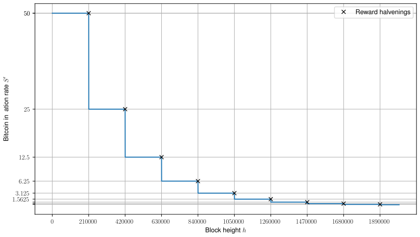Bitcoin inflation rate versus block height.

We can directly compute inflation curvature:

\[S''(h) = \begin{cases} \frac{\ln(\alpha)}{\beta} \alpha^{h/\beta} & \text{if}\quad h\ \mathrm{mod}\ \beta = 0 \quad\text{and}\quad h > 0\\ 0 & \text{otherwise}. \end{cases}\]

$S’’$ is nonzero only when $h$ is a multiple of $\beta$. For $0 < \alpha < 1$, $S’’$ is either zero or negative, which is the case for Bitcoin.

Finally, we can come up with a closed-form $S$ by solving the initial value problem (1):

\[\begin{aligned} S(h) &= \sum_{i=0}^{\lfloor h/\beta\rfloor -1} \alpha^{i} \beta R_0 + \alpha^{\lfloor h/\beta\rfloor} (h\ \mathrm{mod}\ \beta) R_0 \\ &= R_0 \left(\beta\frac{1-\alpha^{\lfloor h/\beta\rfloor}}{1-\alpha} +\alpha^{\lfloor h/\beta\rfloor} (h\ \mathrm{mod}\ \beta) \right) \end{aligned}\]

Here is what the supply function looks like for Bitcoin:

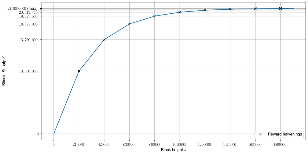Bitcoin supply versus block height.

And the maximum number of Bitcoins to ever exist are calculated by taking the limit

\[\lim_{h\to\infty} S(h) = \sum_{i=0}^{\infty} \alpha^{i} \beta R_0 = \frac{\beta R_0}{1-\alpha} = 21,000,000\text{ BTC}.\]

Summary

The concept of inflation curvature was introduced. The confusion regarding Bitcoin’s inflation mechanism was cleared with an analogy. The IVP defining Bitcoin’s supply was introduced and solved to get a closed-form expression. Inflation curvature for Bitcoin was derived. The maximum number of Bitcoins to ever exist was derived and computed.

Because $S$ is defined over positive integers. ↩

Entries for February 2019

Scalable Reward Distribution with Changing Stake Sizes

Conclusion

Bitcoin's Inflation

Summary