Ethereum is a platform for distributed computing that uses a blockchain for data storage, thus inheriting the many benefits blockchain systems enjoy, such as decentralization and permissionlessness. It also inherited the idea of users paying nodes a fee to get their transactions included in the blockchain. After all, computation on the blockchain is not an infinite resource, and it should be allocated to users who actually find value in it. Otherwise, a feeless blockchain can easily be spammed and indefinitely suffer a denial-of-service attack.

Blockchain state advances on a block by block basis. On a smart contract platform, the quantity of computation as a resource is measured in terms of the following factors:

• Bandwidth: The number of bits per unit time that the network can achieve consensus on.
• Computing power: The average computing power of an individual node.
• Storage: The average storage capacity of an individual node.

The latter two are of secondary importance, because the bottleneck for the entire network is not the computing power or storage capacity of an individual node, but the overall speed of communicating the result of a computation to the entire network. In Bitcoin and Ethereum, that value is around 13 kbps¹, calculated by dividing average full block size by average block time. Trying to increase that number, either by increasing the maximum block size or decreasing block time, indeed results in increased computational capacity. However it also increases the uncle rate², thereby decreasing the quality of consensus—a blockchain’s main value proposition.

Moreover, users don’t just submit bits in their transactions. In Bitcoin, they submit inputs, outputs, amounts etc³. In Ethereum, they can just submit a sender and a receiver of an amount of ETH, or they can also submit data, which can be an arbitrary message, function call to a contract or code to create a contract. This data, which alters Ethereum’s world state, is permanently stored on the blockchain.

Ethereum is Turing complete, and users don’t know when and in which order miners will include their transactions. In other words, users have no way of predicting with 100% accuracy the total amount of computational resources their function call will consume, if that call depends on the state of other accounts or contracts⁴. Furthermore, even miners don’t know it up until the point they finish executing the function call. This makes it impractical for users to set a lump sum fee that they are willing to pay to have their transaction included, because a correlation between a transaction’s fee and its utilization of resources cannot be ensured.

To solve this problem, Ethereum introduced the concept of gas as a unit of account for the cost of resources utilized during transaction execution. Each instruction featured in the Ethereum Virtual Machine has a universally agreed cost in gas, proportional to the scarcity of the used resource⁵. Then instead of specifying a total fee, users submits a gas price in ETH and the maximum total gas they are willing to pay.

The costliest operations on Ethereum are those of non-volatile storage and access⁶, but these need not occupy space in a block. It’s the transactions themselves that are stored in the blocks and thus consume bandwidth. The gas corresponding to this consumption is called “intrinsic gas” (see the Yellow Paper), and it’s one of the reasons for the correlation between gas usage and block size:

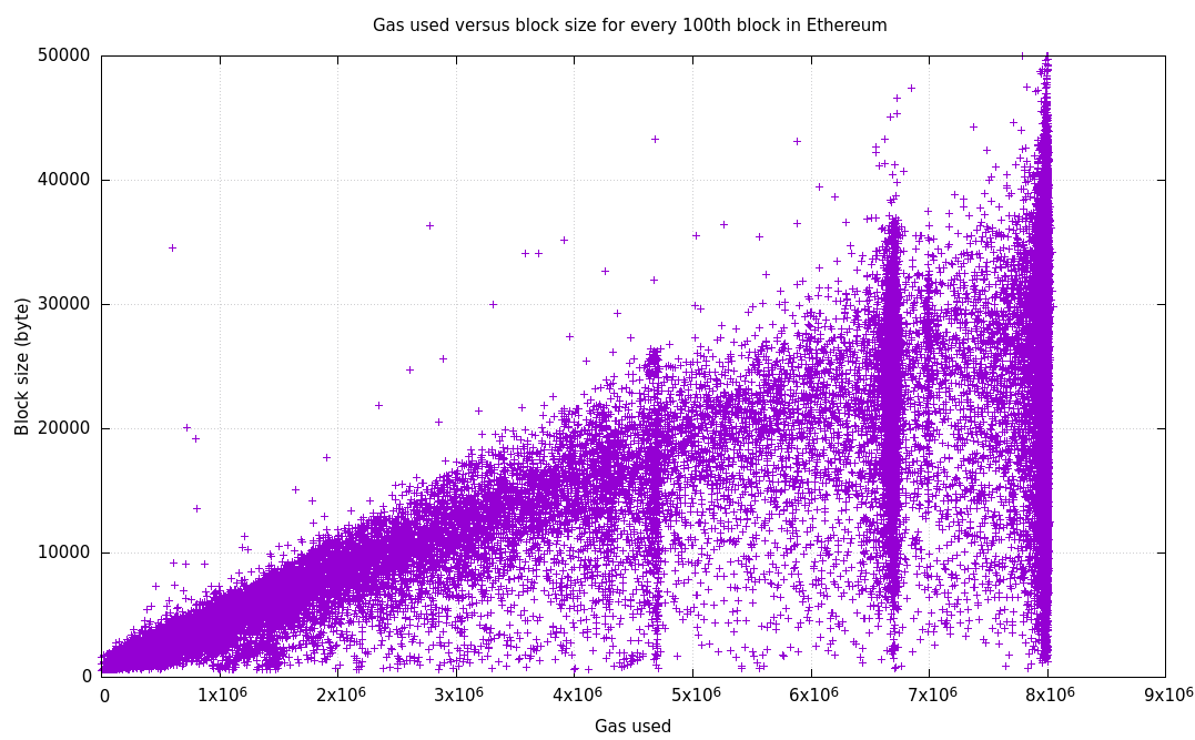
The vertical clusterings at 4.7m, 6.7m and 8m gas correspond to current and previous block gas limits. Gas costs of instructions should indeed be set in such a way that the correlation between a resource and overall gas usage should increase with the degree of bottleneck.

Gas Supply and Demand

The demand for transacting/computing on creates its own market, both similar and dissimilar to the markets of tangible products that we are used to. What is more important to us is the supply characteristics of this market. Supplied quantities aren’t derived from individual capacities and decisions of the miners, but from network bottlenecks. A limit is set on maximum gas allowed per block.

Supplied quantity is measured in terms of gas supplied per unit time, similar to bandwidth. Individual miners contribute hashrate to the network, but this doesn’t affect throughput. The difficulty adjustment mechanism ensures that network throughput remains the same, unless universally agreed parameters are changed by collective decision.

Moreover, the expenditure of mining a block far exceeds the expenditure of executing a block. In other words, changes in overall block fullness doesn’t affect miner operating expenses. Therefore, marginal cost is roughly zero, up until the point supply hits maximum throughput—where blocks become 100% full. At that point, marginal cost becomes infinite. This is characterized by a vertical supply curve located at maximum throughput, preceded by a horizontal supply curve.

This means that given a generic monotonically decreasing demand curve and a certain shift in demand, we can predict the change in the gas price, and vice versa. The price is located at the point where the demand curve intersects the supply curve. Major shifts in price starts to occur only when blocks become full. Past that point, users are basically bidding higher and higher prices to get their transactions included. See the figure below for an illustration.

This sort of econometric analysis can be done simply by looking at block statistics. Doing so reveals 2 types of trends in terms of period:

• Intraday volatility: Caused by shifts in demand that repeat periodically every day.
• Long term shifts: Caused by increases or decreases in the level of adoption, and not periodic.

Note: This view of the market ignores block rewards, but that is OK in terms of analyzing gas price volatility, because block rewards remain constant for very long periods of time. However, a complete analysis would need to take block rewards into account, because they constitute the majority of miner revenue.

Daily Demand Cycle and Intraday Volatility

Demand for gas isn’t distributed equally around the globe. Ethereum users exist in every inhabited continent, with the highest demand seen in East Asia, primarily China. Europe+Africa and the Americas seem to be hand in hand in terms of demand. This results in predictable patterns that follow the peaks and troughs of human activity in each continent. The correlation between gas usage and price is immediately noticeable, demonstrated by a 5 day period from March 2019.

The grid marks the beginnings of the days in UTC, and the points in the graph correspond to hourly averages, calculated as:

• Average hourly gas usage per block = Total gas used in an hour / Number of blocks in an hour
• Average hourly gas price = Total fees collected in an hour / Total gas used in an hour

Averaging hourly gives us a useful benchmark to compare, because block-to-block variation in these attributes is too much for an econometric analysis.

One can see above that the average gas price can change up to 2 to 4 times in a day. This shows us that Ethereum has found real use around the world, but also that there exists a huge UX problem in terms of gas prices.

Dividing the maximum gas price in a day by the minimum, we obtain a factor of intraday volatility:

Ethereum has witnessed gas price increases of up to 100x in a day. Smoothing out the data, we can see that the gas price can change up to 4x daily on average.

To understand the effect of geographic distribution on demand, we can process the data above to obtain a daily profile for gas usage and price. We achieve this by dividing up the yearly data set into daily slices, and standardizing each slice in itself. Then the slices are superimposed and their mean is calculated. The mean curve, though not numerically accurate, makes sense in terms of ordinal difference between the hours of an average day.

One can clearly see that gas usage and price are directly correlated. At 00:00 UTC, it’s been one hour since midnight in Central Europe, but that’s no reason for a dip in demand—China just woke up. The first dip is seen at 03:00 when the US is about to go to sleep, but then Europe wakes up. The demand dips again after 09:00, but only briefly—the US just woke up. We then encounter the biggest dip from 15:00 to 23:00 as China goes to sleep.

Surely there must be a way to absorb this volatility! Solving this problem would greatly improve Ethereum’s UX and facilitate even greater mainstream adoption.

Long Term Shifts in Demand

The long term—i.e. $\gg$ 1 day—shifts in demand are unpredictable and non-periodic. They are caused by adoption or hype for certain applications or use cases on Ethereum, like

• ICOs,
• decentralized exchanges,
• DAI and CDPs,
• interest bearing Dapps,
• games such as Cryptokitties and FOMO3D,
• and so on.

These shifts in price generally mirror ETH’s own price. In fact, it’s not very objective to plot a long term gas price graph in terms of usual Gwei, because most people submit transactions considering ETH’s price in fiat. For that reason, we denote gas price in terms of USD per one million gas, and plot it on a logarithmic scale:

The price of gas has seen an increase of many orders of magnitude since the launch of the mainnet. The highest peak corresponds to the beginning of 2018 when the ICO bubble burst, similar to the price of ETH. Although highly critical for users and traders, this sort of price action is not very useful from a modeling perspective.

Conclusion

The volatility in gas price stems from the lack of scalability. In 2019 on Ethereum, daily gas price difference stayed over 2x on average. The cycle’s effect is high enough to consider it as a recurring phenomenon that requires its own solution.

I think the narrative that gas price volatility is caused only by the occasional game/scam hype is incomplete—in a blockchain that has gained mainstream adoption such as Ethereum, the daily cycle of demand by itself is enough to cause volatility that harms the UX for everyone around the globe.

While increasing scalability is the ultimate solution, users may still benefit from mechanisms that allow them to hedge themselves against price increases, like reserving gas on a range of block heights. This would make a good topic for a future post.

A cryptoeconomic network is a network where

• nodes perform tasks that are useful to the network,
• incur costs while doing so,
• and get compensated through fees paid by the network users, or rewards generated by the network’s protocol (usually in the form of a currency native to the network).

Reward generation causes the supply of network currency to increase, resulting in inflation. Potential nodes are incentivized to join the network because they see there is profit to be made, especially if they are one of the early adopters. This brings the notion of a “cake” being shared among nodes, where the shares get smaller as the number of nodes increases.

Since one of the basic properties of a currency is finite supply, a sane protocol cannot have the rewards increase arbitrarily with more nodes. Thus the possible number of nodes is finite, and can be calculated using costs and rewards, given that transaction fees are negligible. The rate by which rewards are generated determines the sensitivity of network size to changes in costs and other factors.

Let $N$ be the number of nodes in a network, which perform the same work during a given period. Then we can define a generalized reward per node, introduced by Buterin¹:

where $R_0$ is a constant and $\alpha$ is a parameter adjusting how the rewards scale with $N$.

Then the total reward issued is equal to

The value of $\alpha$ determines how the rewards scale with $N$:

Below is a table showing how different values of $\alpha$ corresponds to different rewarding schemes, given full participation.

The case $\alpha \leq 0$ results in unlimited network growth, causes runaway inflation and is not feasible. The case $\alpha > 1$ is also not feasible due to drastic reduction in rewards. The sensible range is $0 < \alpha \leq 1$, and we will explore the reasons below.

Estimating Network Size

We relax momentarily the assumption that nodes perform the same amount of work. The work mentioned here can be the hashing power contributed by a node in a PoW network, the amount staked in a PoS network, or the measure of dedication in any analogous system.

Let $w_i$ be the work performed by node $i$. Assuming that costs are incurred in a currency other than the network’s—e.g. USD—we have to take the price of the network currency $P$ into account. The expected value of $i$’s reward is calculated analogous to (1)

Introducing variable costs $c_v$ and fixed costs $c_f$, we can calculate $i$’s profit as

Assuming every node will perform work in a way to maximize profit, we can estimate $w_i$ given others’ effort:

In a network where nodes have identical costs and capacities to work, all $w_j$ $j=1,\dots,N$ converge to the same equilibrium value $w^\ast$. Equating $w_i=w_j$, we can solve for that value:

Plugging $w^\ast$ back above, we can calculate $N$ for the case of economic equilibrium where profits are reduced to zero due to perfect competition:

which yields the following implicit equation

It is a curious result that for the idealized model above, network size does not depend on variable costs. In reality, however, we have an uneven distribution of all costs and work capacities. Nevertheless, the idealized model can still yield rules of thumb that are useful in protocol design.

An explicit form for $N$ is not possible, but we can calculate it for different values of $\alpha$. For $\alpha=1$, we have

as demonstrated by Thum².

For $0<\alpha<1$, the explicit forms would take too much space. For brevity’s sake, we can approximate $N$ by

given $N \gg 1$. The closer $\alpha$ to zero, the better the approximation.

We also have

which shows that for $\alpha\leq 0$, the network grows without bounds and render the network currency worthless by inflating it indefinitely. Therefore there is no equilibrium.

For $\alpha > 1$, rewards and number of nodes decrease with increasing $\alpha$. Finally, we have

given that transaction fees are negligible.

For $0 <\alpha \ll 1$, a $C$x change in underlying factors will result in $C^{1/\alpha}$x change in network size. For $\alpha=1$, the change will be $\sqrt{C}$x.

Let $\alpha=1$. Then a $2$x increase in price or rewards will result in a $\sqrt{2}$x increase in network size. Conversely, a $2$x increase in fixed costs will result in $\sqrt{2}$x decrease in network size. If we let $\alpha = 1/2$, a $2$x change to the factors result in $4$x change in network size, and so on.

References

This post is an addendum to the excellent paper Scalable Reward Distribution on the Ethereum Blockchain by Batog et al.¹ The outlined algorithm describes a pull-based approach to distributing rewards proportionally in a staking pool. In other words, instead of pushing rewards to each stakeholder in a for-loop with $O(n)$ complexity, a mathematical trick enables keeping account of the rewards with $O(1)$ complexity and distributing only when the stakeholders decide to pull them. This allows the distribution of things like rewards, dividends, Universal Basic Income, etc. with minimal resources and huge scalability.

The paper by Bogdan et al. assumes a model where stake size doesn’t change once it is deposited, presumably to explain the concept in the simplest way possible. After the deposit, a stakeholder can wait to collect rewards and then withdraw both the deposit and the accumulated rewards. This would rarely be the case in real applications, as participants would want to increase or decrease their stakes between reward distributions. To make this possible, we need to make modifications to the original formulation and algorithm. Note that the algorithm given below is already implemented in PoWH3D.

In the paper, the a $\text{reward}_t$ is distributed to a participant $j$ with an associated $\text{stake}_j$ as

where subscript $t$ denotes the values of quantities at distribution of reward $t$ and $T$ is the sum of all active stake deposits.

Since we relax the assumption of constant stake, we rewrite it for participant $j$’s stake at reward $t$:

Then the total reward participant $j$ receives is calculated as

Note that we can’t take stake out of the sum as the authors did, because it’s not constant. Instead, we introduce the following identity:

Identity: For two sequences $(a_0, a_1, \dots,a_n)$ and $(b_0, b_1, \dots,b_n)$, we have

Proof: Substitute $b_i = \sum_{j=0}^{i}b_j - \sum_{j=0}^{i-1}b_j$ on the LHS. Distribute the multiplication. Modify the index $i \leftarrow i-1$ on the first term. Separate the last element of the sum from the first term and combine the remaining sums since they have the same bounds. $\square$

We assume $n+1$ rewards represented by the indices $t=0,\dots,n$, and apply the identity to total reward to obtain

We make the following definition:

and define the change in stake between rewards $t-1$ and $t$:

Then, we can write

This result is similar to the one obtained by the authors in Equation 5. However, instead of keeping track of $\text{reward_per_token}$ at times of deposit for each participant, we keep track of

In this case, positive $\Delta \text{stake}$ corresponds to a deposit and negative corresponds to a withdrawal. $\Delta \text{stake}_{j,t}$ is zero if the stake of participant $j$ remains constant between $t-1$ and $t$. We have

The modified algorithm requires the same amount of memory, but has the advantage of participants being able to increase or decrease their stakes without withdrawing everything and depositing again.

Furthermore, a practical implementation should take into account that a participant can withdraw rewards at any time. Assuming $\text{reward_tally}_{j,n}$ is represented by a mapping reward_tally[] which is updated with each change in stake size

reward_tally[address] = reward_tally[address] + change * reward_per_token

we can update reward_tally[] upon a complete withdrawal of $j$’s total accumulated rewards:

reward_tally[address] = stake[address] * reward_per_token

which sets $j$’s rewards to zero.

A basic implementation of the modified algorithm in Python is given below. The following methods are exposed:

• deposit_stake to deposit or increase a participant stake.
• distribute to fan out reward to all participants.
• withdraw_stake to withdraw a participant’s stake partly or completely.
• withdraw_reward to withdraw all of a participant’s accumulated rewards.

Caveat: Smart contracts use integer arithmetic, so the algorithm needs to be modified to be used in production. The example does not provide a production ready code, but a minimal working example to understand the algorithm.

class PullBasedDistribution:
    "Constant Time Reward Distribution with Changing Stake Sizes"

    def __init__(self):
        self.total_stake = 0
        self.reward_per_token = 0
        self.stake = {}
        self.reward_tally = {}

    def deposit_stake(self, address, amount):
        "Increase the stake of `address` by `amount`"
        if address not in self.stake:
            self.stake[address] = 0
            self.reward_tally[address] = 0

        self.stake[address] = self.stake[address] + amount
        self.reward_tally[address] = self.reward_tally[address] + self.reward_per_token * amount
        self.total_stake = self.total_stake + amount

    def distribute(self, reward):
        "Distribute `reward` proportionally to active stakes"
        if self.total_stake == 0:
            raise Exception("Cannot distribute to staking pool with 0 stake")

        self.reward_per_token = self.reward_per_token + reward / self.total_stake

    def compute_reward(self, address):
        "Compute reward of `address`"
        return self.stake[address] * self.reward_per_token - self.reward_tally[address]

    def withdraw_stake(self, address, amount):
        "Decrease the stake of `address` by `amount`"
        if address not in self.stake:
            raise Exception("Stake not found for given address")

        if amount > self.stake[address]:
            raise Exception("Requested amount greater than staked amount")

        self.stake[address] = self.stake[address] - amount
        self.reward_tally[address] = self.reward_tally[address] - self.reward_per_token * amount
        self.total_stake = self.total_stake - amount
        return amount

    def withdraw_reward(self, address):
        "Withdraw rewards of `address`"
        reward = self.compute_reward(address)
        self.reward_tally[address] = self.stake[address] * self.reward_per_token
        return reward

# A small example
addr1 = 0x1
addr2 = 0x2

contract = PullBasedDistribution()

contract.deposit_stake(addr1, 100)
contract.distribute(10)

contract.deposit_stake(addr2, 50)
contract.distribute(10)

print(contract.withdraw_reward(addr1))
print(contract.withdraw_reward(addr2))

Conclusion

With a minor modification, we improved the user experience of the Constant Time Reward Distribution Algorithm first outlined in Batog et al., without changing the memory requirements.

New bitcoins are minted with every new block in the Bitcoin blockchain, called “block rewards”, in order to incentivize people to mine and increase the security of the network. This inflates Bitcoin’s supply in a predictable manner. The inflation rate halves every 4 years, decreasing geometrically.

There have been some confusion of the terminology, like people calling Bitcoin deflationary. Bitcoin is in fact not deflationary—that implies a negative inflation rate. Bitcoin rather has negative inflation curvature: Bitcoin’s inflation rate decreases monotonically.

An analogy from elementary physics should clear things up: Speaking strictly in terms of monetary inflation,

• displacement is analogous to inflation/deflation, as in total money minted/burned, without considering a time period. Dimensions: $[M]$.
• Velocity is analogous to inflation rate, which defines total money minted/burned in a given period. Dimensions: $[M/T]$.
• Acceleration is analogous to inflation curvature, which defines the total change in inflation rate in a given period. Dimensions: $[M/T^2]$.

Given a supply function $S$ as a function of time, block height, or any variable signifying progress,

• inflation is a positive change in supply, $\Delta S > 0$, and deflation, $\Delta S < 0$.
• Inflation rate is the first derivative of supply, $S’$.
• Inflation curvature is the second derivative of supply, $S’’$.

In Bitcoin, we have the supply as a function of block height: $S:\mathbb{Z}_{\geq 0} \to \mathbb{R}_+$. But the function itself is defined by the arithmetic¹ initial value problem

where $R_0$ is the initial inflation rate, $\alpha$ is the rate by which the inflation rate will decrease, $\beta$ is the milestone number of blocks at which the decrease will take place, and $\lfloor \cdot \rfloor$ is the floor function. In Bitcoin, we have $R_0 = 50\text{ BTC}$, $\alpha=1/2$ and $\beta=210,000\text{ blocks}$. Here is what it looks like:

We can directly compute inflation curvature:

$S’’$ is nonzero only when $h$ is a multiple of $\beta$. For $0 < \alpha < 1$, $S’’$ is either zero or negative, which is the case for Bitcoin.

Finally, we can come up with a closed-form $S$ by solving the initial value problem (1):

Here is what the supply function looks like for Bitcoin:

And the maximum number of Bitcoins to ever exist are calculated by taking the limit

Summary

The concept of inflation curvature was introduced. The confusion regarding Bitcoin’s inflation mechanism was cleared with an analogy. The IVP defining Bitcoin’s supply was introduced and solved to get a closed-form expression. Inflation curvature for Bitcoin was derived. The maximum number of Bitcoins to ever exist was derived and computed.