Entries for 2024

AGI is what generates evolutionarily fit and novel information
I had this idea while taking a shower and felt that I had to share it. It most likely has flaws, so I would appreciate any feedback at onur@solmaz.io. My hunch is that it could be a stepping stone towards something more fundamental.
As the world heads towards Artificial General Intelligence—AGI—people rush to define what it is. Marcus Hutter historically described it as
AI which is able to match or exceed human intelligence in a wide class of environments
(…)
hypothetical agent that can perform virtually all intellectual tasks as well as a typical human could
(see his most recently published book)
whereas OpenAI historically described it as
a highly autonomous system that outperforms humans at most economically valuable work
and more recently, according to a The Information report
an AI system that can generate at least $100 billion in profits for OpenAI
which apparently could be the threshold at which Microsoft loses access to OpenAI models, according to the legal agreement between OpenAI and Microsoft.
Acknowledging all of this and other possible definitions, I want to introduce a definition of AGI that relates to information theory and biology, which I think could make sense:
An AGI is an autonomous system that can generate out-of-distribution (i.e. novel) information, that can survive and spread in the broader environment, at a rate higher than a human can generate.
Here, “survival” can be thought of as mimetic survival, where an idea or invention keeps getting replicated or referenced instead of being deleted or forgotten. Some pieces of information, like blog posts auto-generated for SEO purposes, can quickly vanish, are ephemeral and so recently have started being called “AI slop”. Others, such as scientific theories, math proofs, books such as Euclid’s Elements, and so on, can persist across millennia because societies find them worth copying, citing, or archiving. They are Lindy.
In that way, it is possible to paraphrase the above definition as “an autonomous system that can generate novel and Lindy information at a rate higher than a human can do”.
Like Hutter’s definition, the concept of environment is crucial for this definition. Viruses thrive in biological systems because cells and organisms replicate them. Digital viruses exploit computers. Euclid’s Elements thrives in a math-loving environment. In every case, the information’s persistence depends not just on its content but also on whether its environment considers it worth keeping. This applies to AI outputs as well: if they provide correct or valuable solutions, they tend to be stored and re-used, whereas banal or incorrect results get deleted.
The lifetime of information
Mexican cultural tradition of Día de los Muertos and the anime One Piece have a similar concept on death:
When do you think people die? Is it when a bullet from a pistol pierces their heart? (…) No! It’s when they are forgotten by others! (—Dr. Hiriluk, One Piece)
You could call this specific type of death “informational death”. A specific information, a bytestream representing an idea, a theory, a proof, a book, a blog post, etc., is “dead” when its every last copy is erased from the universe, or cannot be retrieved in any way. Therefore, it is also possible to call a specific information “alive” when it is still being copied or referenced.
So, how could we formalize the survival of information? The answer is to use survival functions, a concept used in many fields, including biology, epidemiology, and economics.
Let us assume that we have an entity, an AI, that produces a sequence of information $x_1, x_2, \ldots, x_n$. For each piece of information $x_i$ produced by the AI, we define a random lifetime $T_i \ge 0$. $T_i$ is the time until $x_i$ is effectively forgotten, discarded, or overwritten in the environment.
We then describe the survival function as:
\[S_i(t) = \mathbb{P}[T_i > t],\]the probability that $x_i$ is still alive (stored, referenced, or used) at time $t$. This is independent of how many duplicates appear—we assume that at least one copy is enough to deem it alive.
In real life, survival depends on storage costs, attention spans, and the perceived value of the item. A short-lived text might disappear as soon as nobody refers to it. A revolutionary paper may endure for decades. Mathematical facts might be considered so fundamental that they become permanent fixtures of knowledge. When we speak of an AI that “naturally” produces persistent information, we are observing that correct or notable outputs often survive in their environment without the AI having to optimize explicitly for that outcome.
An expanding universe of information
In our definition above, we mention “out-of-distribution”ness, or novelty of information. This implies the existence of a distribution of information, i.e. a set of information containing all information that has ever been generated up to a certain time. We denote this set of cumulative information as $U$ for “universe”, which grows with every new information $x_i$ produced by the AI. Let
\[U_0 \quad \text{be the initial "universe" (or data) before any } x_i \text{ is introduced,}\]and then
\[U_{i+1} = U_{i} \cup \{x_{i+1}\} \quad\text{for } i=1,\dots,N.\]In other words, once $x_{i+1}$ is added, it becomes part of the universe. Given an existing state of $U_i$, we can define and calculate a “novelty score” for a new information $x_{i+1}$ relative to $U_i$. If $x_{i+1}$ is basically a duplicate of existing material, its novelty score will be close to zero. If it is genuinely out-of-distribution, it would be large. Therefore, when a novel information $x_{i+1}$ is added to $U$, any future copies of it will be considered in-distribution and not novel. We denote the novelty score of $x_{i+1}$ as $n_{i+1}$.
So how could we calculate this novelty score? One way to calculate it is to use conditional Kolmogorov complexity:
\[n_{i+1} = K(x_{i+1} | U_i)\]where
\[K(x | U) = \min_{p} \Bigl\{ \lvert p \rvert : M(p, U) = x \Bigr\}.\]is the length (in bits) of the shortest program that can generate $x$, when the set $U$ is given as as a free side input, and $M$ is the universal Turing machine.
How does this relate to novelty?
Low novelty: If $x$ can be produced very easily by simply reading or slightly manipulating $U$, then the program $p$ (which transforms $U$ into $x$) is small, making $K(x \mid U)$ and hence the novelty score is low. We would say that $x$ is almost already in $U$, or is obviously derivable from $U$.
High novelty: If $x$ shares no meaningful pattern with $U$, or can’t easily be derived from $U$, the program $p$ must be large. In other words, no short set of instructions that references $U$ is enough to produce $x$—it must encode substantial new information not present in $U$. That means $K(x \mid U)$ and hence the novelty score is high.
Informational fitness
We can now combine survival and novelty to formalize our informal definition of AGI-ness above. We integrate the survival function over time to the expected lifetime of information $x_i$:
\[L_i = \int_{0}^{\infty} S_i(t)\,\mathrm{d}t = \mathbb{E}[T_i].\]Therefore, for an entity which generates information ${x_1, x_2, \ldots, x_n}$ over its entire service lifetime, we can compute a measure of “informational fitness” by multiplying the novelty score $n_i$ by the expected lifetime $L_i$ over all generated information:
\[\boxed{\text{IF} = \sum_{i=1}^n w_i L_i.}\]This quantity tracks the total sum of both how novel each new piece of information an entity generates, and how long it remains in circulation.
My main idea is that a higher Informational Fitness would point to a higher ability to generalize, and hence a higher level of AGI-ness.
Because each subsequent item’s novelty is always measured with respect to the updated universe that includes all prior items, any repeated item gets a small or zero novelty score. Thus, it doesn’t inflate the overall Informational Fitness measure.
Why worry about novelty at all? My concern came from viruses, which are entities that copy themselves and spread, and therefore could be considered as intelligent if we simply valued how many times an information is copied. But viruses are obviously not intelligent—they mutate randomly and any novelty comes from selection by the environment. Therefore, a virus itself does not have a high IF in this model. However, an AI that can generate many new and successful viruses would indeed have a high IF.
Information’s relevance
Tying AGI-ness to survival of information renders the perception of generalization ability highly dependent on the environment, or in other words, state of the art at the time of an AI’s evaluation. Human societies (and presumably future AI societies) advance, and the window of what information is worth keeping drifts over time, erasing the information of the past. So whereas an AI of 2030 would have a high IF during the years it is in service, the same system (same architecture, training data, weights) would likely have a lower IF in 3030, due to being “out of date”. Sci-fi author qntm has named this “context drift” in his short story about digitalized consciousness.
Comparing AI with humans
Humans perish with an expected lifetime of 80 years, whereas AI is a digital entity that could survive indefinitely. Moreover, if you consider an AI’s performance depends on the hardware it runs on, you realize that IF should be derived from the maximum total throughput of all the copies of the AI that are running at a time. Basically, all the information that is generated by that specific version of the AI in the entire universe counts towards its IF.
Given this different nature of AI and humans, how fair would it be to compare a human’s informational fitness with an AI’s? After all, we cannot digitize and emulate a human’s brain with 100% fidelity with our current technology, and a fair comparison would require exactly that. We then quickly realize that we need to make assumptions and use thought experiments, like hypothetically scanning the brain of Albert Einstein (excuse the cliché) and running it at the same bitrate and level of parallelism as e.g. OpenAI’s most advanced model at the time. Or we could consider the entire thinking power of the human society as a whole and try to back-of-the-envelope-calculate that from the number of Universities and academics. But given that a lot of these people already use AI assistants, how much of their thinking would be 100% human?
The original OpenAI definition “a highly autonomous system that outperforms humans at most economically valuable work” is a victim of this as well. Humans are using AI now and are becoming more dependent on it, and smarter at the same time. Until we see an AI system that is entirely independent of human input, it will be hard to draw the line in between human and AI intelligence.
Thank you for reading up to this point. I think there might be a point in combining evolutionary biology with information theory. I tried to keep it simple and not include an information’s copy-count in the formulation, but it might be a good next step. If you think this post is good or just dumb, you can let me know at onur@solmaz.io.
-
-
-
-
Our muscles will atrophy as we climb the Kardashev Scale
If you like this, you might also like my Instagram channel Nerd on Bars @nerdonbars where I calculate the power output of various athletes and myself.
This is an addendum to my previous post The Kilowatt Human. I mean it as half-entertainment and half-futuristic speculation. I extrapolate the following insight more into the future:
Before the industrial revolution, over 80% of the population were farmers. The average human had to do physical labor to survive. The average human could not help but to “bodybuild”.
Since then, humans have built machines to harness the power of nature and do the physical labor for them. What made the human civilization so powerful robbed individual humans of their own power, quite literally. The average pre-industrial human could generate a higher wattage than the average post-industrial human of today—they had to.
Before the industrial revolution, humanity’s total power output was bottlenecked by human physiology. Humanity has since moved up in the Kardashev scale. Paradoxically, the more power humanity can generate, the less physical exercise the average human can economically afford, and the weaker their body becomes.
Similar to the growth in humanity’s energy consumption, the average human’s physical strength will move down a spectrum, marked by distinct Biomechanical Stages, or BMS for short:
Biomechanical Stage Technology Level Human Physical Labor Biomechanical Power Condition BMS-I (Pre-Industrial) Stone Age to primitive machinery (sticks, stones, metal tools, mills) Nearly all tasks powered by muscle; farming, hunting, building High: Strength is universal and necessary BMS-II (Industrial-Modern) Steam engines to motorized vehicles Most heavy work done by machines; exercise optional, not required Moderate to Low: Average strength declines as tasks mechanize BMS-III (Post-Biological) Brain chips, quantum telepresence, digital existence Physical labor negligible; teleoperation replaces bodily exertion Nearly None: Muscles vestigial or irrelevant, having a body is comparatively wasteful and an extreme luxury Why do I write this? My father grew up while working as a farmer on the side, then studied engineering. He never did proper strength training in his life. I grew up studying full-time, have been working out on and off, more so in the last couple of years. And I still have a hard time beating him in arm wrestling despite the 40 years of age gap. Our offsprings will be lucky enough if they can afford to have enough time and space to exercise. I hope that their future never becomes as dramatic as I describe below.
Biomechanical Stage I (Pre-Industrial Human Power)
Began with the Stone Age, followed by the era of metal tools, basic mechanical aids like mills, and ended with the industrial revolution:
Stone Age: No metal tools, no machinery. Humans rely on their bodies entirely—hunting, gathering, carrying, and building shelters by hand. Biomechanical power is the cornerstone of survival. The average human can generate and sustain relatively high wattage because everyone is physically active out of necessity. Most humans are hunter-gatherers.
Metal tools and agriculture: Introduction of iron and steel tools improves efficiency in cutting and shaping the environment. Most people farm, carrying heavy loads, tilling fields, harvesting. Though tools reduce some brute force, overall workloads remain high and physically demanding.
Primitive machinery (e.g. mills): Waterwheels and windmills start to handle some repetitive tasks like grinding grain. Still, daily life is labor-intensive for the majority. Physical strength remains a defining human attribute.
In this era, the biomechanical power of the average human is relatively high. The average human can generate and sustain relatively high wattage because everyone is physically active out of necessity.
Biomechanical Stage II (Industrial-Modern Human Power)
We are currently in this stage. It began with the Steam Age, followed by the widespread use of internal combustion engines and motorized vehicles, and will end at the near-future threshold where technology allows a human to be economically competitive and sustain themselves without ever moving their body.
Steam engine and early industry: Factories powered by steam reduce the need for raw human muscle. Some humans shift to repetitive but less physically grueling jobs. Manual labor declines for a portion of the population.
Motorized vehicles and automation (our present): Tractors, trucks, and powered tools handle the heavy lifting. Most humans now work in services or knowledge sectors. The need to exercise for health arises because physical strength no longer follows naturally from daily life. Specialty fields (construction, sports, fitness enthusiasts) maintain higher-than-average output, but they are exceptions.
Humans still have bodies and can choose to train them, but the average sustained power output falls as convenient transport, automation, and energy-dense foods foster sedentary lifestyles.
Robots and AI: Robots and AI are increasingly able to handle physical tasks that were previously done by humans. This further reduces the need for human physical labor.
As machines handle more tasks, the average person’s baseline physical capability drops. Exercise shifts from natural necessity to a personal choice or hobby.
Biomechanical Stage III (Post-Biological Human Power)
Future scenarios where brain-machine interfaces, telepresence, and total virtualization dominate. Will begin with a Sword-Art Online-like scenario where neural interfaces allows a human to remotely control a robot in an economically competitive way, while spending most of their time immobilized. Will end in a Matrix-like scenario where the average human is born as a brain-in-a-jar.
Brain Chips and Teleoperation: Humans remotely control robots with no physical exertion. Commuting is done digitally. Physical strength becomes even less relevant. The population’s average biomechanical output plummets because few move their own bodies meaningfully.
Quantum Entanglement and Zero-Latency Control: Even physical constraints of distance vanish. Humans may spend their entire lives in virtual worlds or controlling machines from afar, further reducing any reason to maintain physical strength.
Bodily Sacrifice, Brains in Jars: Eventually, bodies become optional. Nervous systems are maintained artificially, teleoperating robots when needed. Muscle tissue atrophies until it is nonexistent. The concept of human biomechanical power no longer applies. The definition of what a human is becomes more and more abstract. Is it organic nerve tissue or even just carbon-based life?
The human body, if it exists at all, is not maintained for physical tasks. The average person’s muscular capability collapses to negligible levels.
How does the Kardashev Scale align with the Biomechanical Stages?
In my opinion, the stages will not align perfectly with Kardashev Type I, II and III civilizations. Instead, they will overlap in the following way:
Kardashev Type Biomechanical Stage Description Type I (Planetary) BMS-I (Pre-Industrial) The average human can generate and sustain relatively high wattage because everyone is physically active out of necessity. Most humans are hunter-gatherers or farmers. BMS-II (Industrial-Modern) Humans still have bodies and can choose to train them, but the average sustained power output falls as convenient transport, automation, and energy-dense foods foster sedentary lifestyles. We are still limited to 1 planet. Type II (Interstellar) BMS-III (Post-Biological) The average person’s muscular capability collapses to negligible levels. The concept of human biomechanical power no longer applies. The definition of what a human is becomes more and more abstract. Type III (Galactic) What kind of societal organism can consume energy at a galactic scale? Is there any hope that they will look like us? I think that by the time we reach other stars, we will also have pretty sophisticated telepresence and brain-machine interface technology. In fact, those technologies might be the only way to survive such journeys, or not have to make them at all, as demonstrated in the Black Mirror episode Beyond the Sea:

Black Mirror: Beyond the Sea. Go watch it if you haven’t, it’s the best episode of the season.
So BMS-III might already be here by the time we are a Type II civilization. As for what an organic body means for a Type III galactic civilization, I can’t even begin to imagine.
This post has mostly been motivated by my sadness that while our life quality has increased with technology, it has also decreased in many other ways. We evolved for hundreds of thousands of years to live mobile lives. But we became such a successful civilization that we might soon not be able to afford movement. We are thus in a transitory period where we started to diverge from our natural way of life, too quickly for evolution to catch up. And when evolution finally does catch up, what will that organism look like? How will it feed itself, clean itself and reproduce? Will the future humans be able to survive going outside at all?
In another vein, technology could also help us perfectly fit bodies by altering our cells at a molecular level. But if there is no need to move to contribute to the economy, why would anyone do such an expensive thing?
My hope is that sexual competition and the need for reproduction will maintain an evolutionary pressure just enough to keep our bodies fit. This assumes that individual humans are still in control of their own reproduction and can select their partners freely. Because a brain-in-a-jar is obviously not an in-dividual—they have been divided into their parts and kept only the one that is economically useful.
-
Hi @cursor_ai, if your models could stop removing my painstakingly written comments, that would be great? Ok? Thanks (I know I could define some rules for this or something, but this shouldn't be default behavior)
-
@konradgajdus me reading this book
-
-
The Kilowatt Human
tl;dr: I calculate my power output in Watts/Horsepower and aim to maximize that, instead of muscle volume, in my workouts:
This is a work in progress, email feedback to onur@solmaz.io.
If you like this, you might also like my Instagram channel Nerd on Bars @nerdonbars where I calculate the power output of various athletes and myself.
Why do people hit the gym? What is their goal?
For some, it is to put on muscle and look good. For others, it is to be healthy and live longer. For yet others, it is to have fun, because doing sports is fun. None of these are mutually exclusive.
In this post, I will not focus on any of these. I will focus on the goal of getting strong and building power. I write this, because I feel like people are doing exercise more and more for appearance’s sake, and less to get strong. And it has to do with economics.
Before the industrial revolution, over 80% of the population were farmers. The average human had to do physical labor to survive. The average human could not help but to “bodybuild”.
Since then, humans have built machines to harness the power of nature and do the physical labor for them. What made the human civilization so powerful robbed individual humans of their own power, quite literally. The average pre-industrial human could generate a higher wattage than the average post-industrial human of today—they had to.
Before the industrial revolution, humanity’s total power output was bottlenecked by human physiology. Humanity has since moved up in the Kardashev scale. Paradoxically, the more power humanity can generate, the less physical exercise the average human can economically afford, and the weaker their body becomes. Strength has become a luxury.
This is why most modern fitness terms make me sad, because they remind me of what has been lost.
Consider “functional training”. There used to be no training other than “functional”, because most physical effort had to create economic value. The term is used to differentiate between exercises with machines which target specific muscles, and exercises that are composed of more “compound movements” that mimic real-life activities. It used to be that people did not have to do any training, because physical exercise was already a part of their daily life.
This is why I dislike “building muscle” as a goal as well. Since strength is a luxury now, people want to maximize that in their lives. However, they end up trying to maximize the appearance of strength, because increasing actual strength is harder than building muscle.
When I say it is harder to get strong than to look strong, I mean it in the most materialistic sense: Increasing your body’s power output in Watts is harder and economically more expensive than increasing muscle volume in Cubic Centimeters. Increasing wattage has a higher time and money cost, requires more discipline and a lot more effort. It is a multi-year effort.
Contrarily, muscle can be built quicker in a matter of months, without getting relatively stronger. Many bodybuilders can’t do a few pull-ups with proper form. Their strength doesn’t transfer to other activities. They are sluggish and lack agility. In that sense, bodybuilding culture today embodies the worst parts of capitalism and consumerism. Empty, hollow muscle as a status symbol. Muscle for conspicuous fitness.
To meet up the demand, capitalism has commoditized exercise in the form of the modern machine-laden gym: a cost-optimized low-margin factory. Its product is the ephemeral Cubic Centimeter of Muscle™ which goes away quickly the moment you stop working out.
These gyms are full of people whose main motivation for working out is feeling socially powerless and unattractive. However, instead of going after real physical power, i.e. Watts, they go after the appearance of power, muscle volume. They compare themselves to people that just look bigger, people with higher volume.
The goal of this post is to convince you that it is superior to chase Watts than to chase muscle volume. It is psychologically more rewarding, the muscle gained from it is more permanent and has higher power density. However, it is more difficult and takes longer to achieve.
Goals
Goals matter. For example, if you purely want to maximize your muscle mass or volume, using steroids or questionable supplements is a rational thing to do. Enough people have criticized it such that I don’t need to. Disrupting your hormonal system just to look bigger and be temporarily stronger is extremely dumb.
I personally want to:
- feel powerful, and not just look like it.
- live as long and healthily as I can.
I believe that the best way to do that is to increase my power output in Watts and do regular strength training in a balanced way that will not wear out my body.
If I had to define an objective function for my exercise, it would be:
\[f(P, L) = \alpha P + \beta L(P)\]where $P [\text{Watt}]$ is my power output, $L(P)[\text{year}]$ is the length of my life as a function of my power output, $\alpha$ and $\beta$ are weights that I assign to power and longevity. I won’t detail this any further, because I don’t want to compute anything. I just want to convey my point.
Notice how I don’t constrain myself to any specific type of exercise, such as calisthenics or weightlifting. As long as it makes me more powerful, anything goes. Is wrestling going to get me there? Count me in. Is working in the fields, lifting rocks, firefighter training or Gada training going to get me there? I don’t differentiate. As long as it makes me more powerful, I am in.
Calculating power
How can one even calculate their power output?
It is actually quite easy to do, with high-school level physics. You just need to divide the work done by the time it took.
For example, consider a muscle-up:
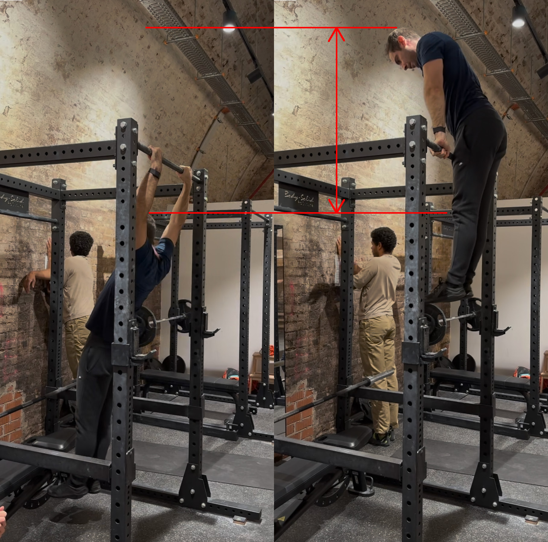
Left: Muscle-up starting position. Right: Top of the movement.
I am at the starting position on the left, and at the top of the movement on the right. In both frames, my velocity is 0, so there is no kinetic energy. Therefore, we can calculate a lower bound of my power output by comparing the potential energies between the two frames. Denoting the left frame with subscript 0 and the right frame with subscript 1, we have:
\[U_0 = mgh_0, \quad U_1 = mgh_1\]where $U$ is the potential energy, $m$ is my mass, $g = 9.81 m/s^2$ is the acceleration due to gravity and $h$ is the height.
The work I do is the change in potential energy:
\[W = U_1 - U_0 = mg(h_1 - h_0) = mg\Delta h\]And my power output is the work divided by the time it took:
\[P = \frac{W}{\Delta t} = \frac{mg\Delta h}{\Delta t}\]The distance I traveled $\Delta h$ can be calculated from anthropometric measurements:
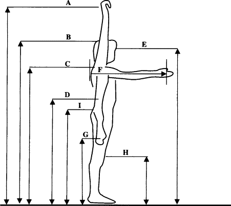
Various distances on the human body.
I will denote the distances from this figure with subscripts $d_A$, $d_B$ and so on. Comparing this with the previous figure, we have roughly:
\[\Delta h \approx d_A - d_G\]To understand how I derive this, consider the hands fixed during the movement and that the body is switching from a position where the arms are extended upwards to a position where the arms are extended downwards.
I have measured my own body, and found this to be roughly equal to 130 cm. Given that it took me roughly 2 seconds to do the movement and my mass at the time was roughly 78 kg, I have found the lower bound of my power output to be:
\[P_{\text{muscleup}} = \frac{mg\Delta h}{\Delta t} = \frac{78 \text{kg} \times 9.81 \text{m/s}^2 \times 1.3 \text{m}}{2 \text{s}} \approx 500 \text{W}\]It is a lower bound, because the muscles are not 100% efficient, some energy is dissipated e.g. as heat during the movement, my movement is not perfectly uniform, etc.
Still, the lower bound calculation is pretty concise, and can be made even more accurate with a stopwatch and a slow-motion camera.
Aiming for 1 kilowatt
When I was first running to calculations, I wanted to get a rough idea of the order of magnitude of the power output of various exercises. It surprised me when I found out that most exercises are in 10-1000 Watt range, expressable without an SI prefix.
I have been training seriously for almost a year and regularly for a couple of years before that. I have discovered that in my current state, my unweighted pull-ups are in the 500-1000 Watt range. For the average person, 1000 Watts, i.e. 1 kilowatt, is an ambitious goal, but not an unattainable one. 1 kilowatt simply sounds cool as a target to aim for, as if you are a dynamo, a machine. A peak athlete can easily generate 1 kilowatt with their upper body for short durations.
How does this reflect to the muscle-up example I gave above?
If I am not adding any additional weights to my body, that means the duration which I complete the movement would need to decrease. We can calculate how much that would need to be. Moreover, we can derive a general formula which calculates how fast anyone would need to perform a muscle-up to generate 1 kilowatt.
To do that, we first need to express power in terms of the person’s height. Previously, we had $\Delta h = d_A - d_G$. Most people have roughly similar anthropometric ratios, so we can use my measurements to approximate that ratio. Multiply and divide by $d_B$ to get:
\[\Delta h = \frac{d_A - d_G}{d_B} d_B\]For me, $d_A = 215 \text{cm}$, $d_B = 180 \text{cm}$ and $d_G = 85 \text{cm}$, so:
\[\frac{d_A - d_G}{d_B} = \frac{215 \text{cm} - 85 \text{cm}}{180 \text{cm}} \approx 0.722\]Let’s denote the person’s height $d_B$ as $h_p$. Then we have
\[\Delta h = 0.722 h_p\]Therefore, the power output can be expressed as:
\[P \approx 0.722\frac{m g h_p}{\Delta t}\]Since we want to generate 1 kilowatt, we can solve for $\Delta t$:
\[\Delta t = \frac{0.722 m g h_p}{1000}\]If we substitute $g = 9.81 \text{m/s}^2$ and assume $h_p$ is in centimeters, we get roughly:
\[\boxed{ \Delta t_{kilowatt}[\text{s}] \approx \frac{m [\text{kg}] h_p [\text{cm}]}{14000} }\]The formula is really succinct and easy to remember: Just multiply the person’s mass in kilograms by their height in centimeters and divide by 14000.
Calculating for myself, I get $78 \times 180 / 14000 \approx 1.00$ seconds.
This confirms that I need to get two times faster in order to generate 1 kilowatt. Alternatively, if I hit a wall in terms of speed, I could add weights to my body to increase my power output. (TBD)
My friend and trainer J has agreed to record his muscle-up and various other exercises, so I will add his numbers and compare them soon.
TBD: Add the data from J.
Extending to other movements
I chose the muscle-up because I’ve been working on it recently. However, this method can be applied to any movement, as it’s just an application of basic physics.
For example,
- Do you want to calculate the power output of a pull-up? You just need to change the height $\Delta h$, it’s roughly half the distance for muscle-up.
- Do you want to calculate the power output of a weighted pull-up? You just need to add the additional mass to your body mass $m$.
- Do you want to calculate the power output of a sprint start? Just measure your top speed at the beginning and the time it took to accelerate to that speed, and divide your kinetic energy by that time.
- Do you want to calculate the power output of a bench press? You need to set $\Delta h$ as your arm length and $m$ as the weight of the barbell.
See the next section for a more detailed example.
Power-weight relationship in a bench press
In the bodyweight examples above, we had the same bodyweight, and it was being moved over different distances.
Then a good question to ask is: How does the power output scale with the weight lifted? The bench press is an ideal exercise to measure this in a controlled way.
25% slowed down and synced videos of a bench press with increasing weights. Top row left to right: Rounds 1, 2, 3. Bottom row left to right: Rounds 4, 5, 6.
I asked my friend to help me out with timing bench press repetitions over 6 rounds with different weights. You can see these in the video above.
Before we even look at the results, we can use our intuition to guess what kind of relationship we will see. If the weight is low, power is low as well. So as we increase the weight, we expect the power to increase. However, human strength is limited, so the movement will slow down after a certain point, and the power will decrease. We should see the power first increase with weight, and then decrease. This is indeed what happens.
In each round, my friend did 3 to 4 repetitions with the same weight. I calculated the average time it took to complete the repetition and the total weight (barbell + plates) lifted in that round. Then, I calculated the power output for each round using the formula above. The height that the barbell travels during the ascent is $\Delta h = 43 \text{cm}$.
Round Total Weight $m$ (kg) Average Time $\Delta t$ (ms) Power $P$ (Watt) 1 40 580 291 2 45 623 305 3 50 663 318 4 55 723 321 5 60 870 291 6 65 1043 263 The visualizations below are aligned with the intuition:

Total weight vs average time in a bench press. Time taken increases monotonically and super-linearly with weight.

Total weight vs power in a bench press. Power first increases with weight, then decreases.

Average time vs power in a bench press. Similar to the weight vs power plot, but with time on the x-axis.
The figures matches the perceived difficulty of the exercise. My friend said he usually trains with 45-50 kg, and it started to feel difficult in the last 2 rounds. His usual load is under the 55 kg limit where his power saturates. That could mean he is under-loading, and should load at least 60 kg to achieve progressive overload and increase his power.
Reinventing Velocity Based Training, Plyometrics etc.
Power is a factor of speed and force. So in a nutshell, this project is about maximizing speed and force at the same time.
While starting this project, I wanted to have a fresh engineer’s look at powermaxxing, and did not want to get influenced by existing methods or literature. I knew that sports people were using scientific methods to measure and improve performance for decades, but I wanted to discover things on my own. I will continue to stay away from existing knowledge for some time, before I look at them in more detail.
Also: I have personally not seen any person on social media that tracks power output in Watts, or visualizes it with a Wattmeter.
If you know about such a channel, please let me know.
Not-conclusion
This is a work in progress, so there is no conclusion to this yet. I will add more content as I learn more.
Aim for Watts. It is hard, but more rewarding.
-
.@TextCortex AI now uses @astral_sh uv for production builds One of the happiest switches so far, many developer days saved per year
-
-
-
Python might take over JavaScript as the most used language after all uv from @astral_sh is one of the biggest upticks in Python developer experience in the last 10 years I've seen so many people struggle with Python distributions, virtual environments, Anaconda, etc. over the years Most newbies don't care about where their Python executables are, why they have to edit PATH, or why they have to activate a virtual environment It seems like uv has fixed this: https://t.co/lgP5btGrbV
-
3-4 messages back and forth with o1-preview, and I have a CLI tool to remove debug statements from my code. No need to do a search for import ipdb... and manually delete the lines. Instead just run in your project: $ rmdbg . Written in Rust so it's fast https://t.co/yWuF3mDzUC
-
-
This has late 90s Bill Gates/Windows Server vibes tbh Open Thought > Closed Thought
-
Open Thought > Closed Thought
OpenAI released a new model that “thinks” to itself before it answers. They intentionally designed the interface to hide this inner monologue. There was absolutely no technical reason to do so. Only business reasons
If you try to make o1 reveal its inner monologue, they threaten to remove your access
Because if they let people freely extract this, competitors could quickly use that to improve their models
It seems that AI value creation will be shifting more towards inference-time compute, into Chains of Thought. We might be witnessing the birth of a new paradigm of open vs. closed thought
Impressive as o1 is, the move to hide CoTs is pretty pathetic and reminds of Microsoft’s late 90s Windows Server push. Below is an email from Bill Gates about how he is worried that Microsoft won’t be able to corner the server market. A few years after he wrote those lines, Linux and LAMP came to dominate servers
Now all eyes on AI at Meta and Zuck for their take on o1/Strawberry/Q*/Orion


Originally posted on LinkedIn
-
Imagine the following scenario: 1. We develop brain-scan technology today which can take a perfect snapshot of anyone’s brain, down to the atomic level. You undergo this procedure after you die and your brain scan is kept in some fault-tolerant storage, along the lines of GitHub Arctic Code Vault. 2. But sufficiently cheap real-time brain emulation technology takes considerably longer to develop—say 1000 years in the future. 3. 1000 years pass. Everyone that ever knew, loved or cared about you die. Here is the crucial question: Given that running a brain scan still costs money in 1000 years, why should anyone bring *you* back from the dead? Why should anyone boot *you* up? Compute doesn’t grow in trees. It might become very efficient ... (read more in my blog: https://t.co/WCUmzVM4Nu) --- I intended this thought piece as entertainment, almost went to Hacker News frontpage: https://t.co/PnH61jryVa It must have hit some psychological spot, since people wrote a lot of comments, possibly more than number of upvotes.
-
-
Why should anyone boot *you* up?
Imagine the following scenario:
- We develop brain-scan technology today which can take a perfect snapshot of anyone’s brain, down to the atomic level. You undergo this procedure after you die and your brain scan is kept in some fault-tolerant storage, along the lines of GitHub Arctic Code Vault.
- But sufficiently cheap real-time brain emulation technology takes considerably longer to develop—say 1000 years in the future.
- 1000 years pass. Everyone that ever knew, loved or cared about you die.
Here is the crucial question:
Given that running a brain scan still costs money in 1000 years, why should anyone bring *you* back from the dead? Why should anyone boot *you* up?
Compute doesn’t grow in trees. It might become very efficient, but it will never have zero cost, under physical laws.
In the 31st century, the economy, society, language, science and technology will all look different. Most likely, you will not only NOT be able to compete with your contemporaries due to lack of skill and knowledge, you will NOT even be able to speak their language. You will need to take a language course first, before you can start learning useful skills. And that assumes some future benefactor is willing to pay to keep you running before you can start making money, survive independently in the future society.
To give an example, I am a software developer who takes pride in his craft. But a lot of the skills I have today will most likely be obsolete by the 31st century. Try to imagine what an 11th century stonemason would need to learn to be able to survive in today’s society.
1000 years into the future, you could be as helpless as a child. You could need somebody to adopt you, send you to school, and teach you how to live in the future. You—mentally an adult—could once again need a parent, a teacher.
(This is analogous to cryogenics or time-capsule sci-fi tropes. The further in the future you are unfrozen, the more irrelevant you become and the more help you will need to adapt.)
Patchy competence?
On the other hand, it would be a pity if a civilization which can emulate brain scans is unable to imbue them with relevant knowledge and skills, unable to update them.
For one second, let’s assume that they could. Let’s assume that they could inject your scan with 1000 years of knowledge, skills, language, ontology, history, culture and so on.
But then, would it still be you?
But then, why not just create a new AI from scratch, with the same knowledge and skills, and without the baggage of your personality, memories, and emotions?
Why think about this now?
Google researchers recently published connectomics research (click here for the paper) mapping a 1 mm³ sample of temporal cortex in a petabyte-scale dataset. Whereas the scanning process seems to be highly tedious, it can yield a geometric model of the brain’s wiring at nanometer resolution that looks like this:
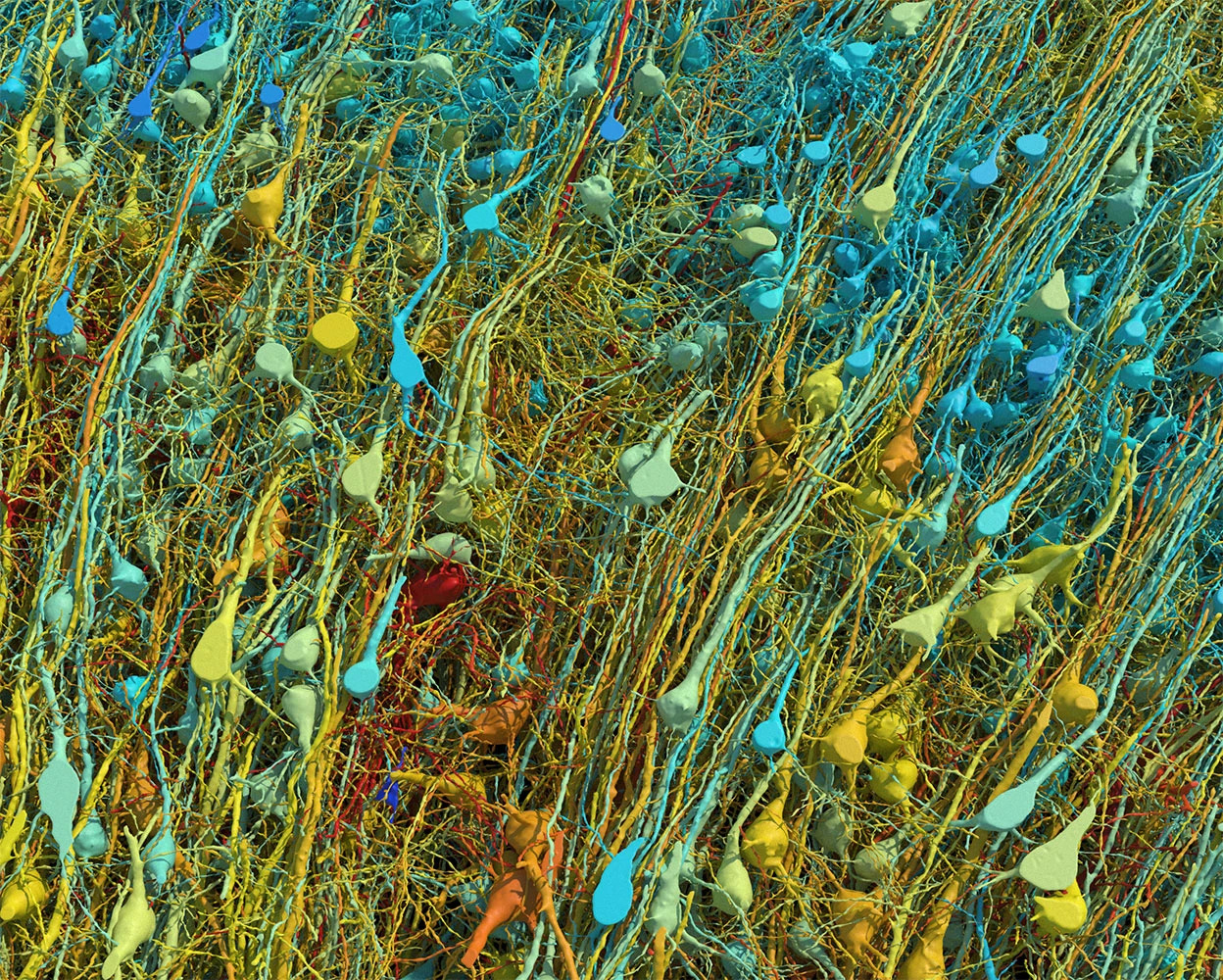
Rendering based on electron-microscope data, showing the positions of neurons in a fragment of the brain cortex. Neurons are coloured according to size. Credit: Google Research & Lichtman Lab (Harvard University). Renderings by D. Berger (Harvard University) They have even released the data to the public. You can download it here.
An adult human brain takes up around 1.2 liters of volume. There are 1 million mm³ in a liter. If we could scale up the process from Google researchers 1 million times, we could scan a human brain at nanometer resolution, yielding more than 1 zettabyte (i.e., 1 billion terabytes) of data with the same rate.
That is an insane amount of data, and it seems infeasible to store that much data for a sufficient number of bright minds, so that this technology can make a difference. That being said, do we have any other choice but to hope that we will find a way to compress and store it efficiently?
Not only it is infeasible to store that much data with current technology, extracting a nanometer-scale connectome of a human brain may not be enough to capture a person’s mind in its entirety. By definition, some information is lost in the process. Fidelity will be among the most important problems in neuropreservation for a long time to come.
That being said, the most important problem in digital immortality may not be technical, but economical. It may not be about how to scan a brain, but about why to scan a brain and run it, despite the lack of any economic incentive.
-
-
Frequencies of Definite Articles in Written vs Spoken German
tl;dr Skip to the Conclusion. Don’t forget to look at the graphs.
Unlike a single “the” in the English language, the German language has 6 definite articles that are used based on a noun’s gender, case and number:
- 6 definite articles: der, die, das, den, dem, des
- 3 genders: masculine, feminine, neuter (corresponding to “he”, “she”, “it” in English)
- 4 cases: nominative, accusative, dative, genitive
- 2 numbers: singular, plural
The following table is used to teach when to use which definite article:
Case Masculine Feminine Neuter Plural Nominative der die das die Accusative den die das die Dative dem der dem den Genitive des der des der Table 1: Articles to use in German depending on the noun gender and case.
Importantly, native speakers don’t look at such tables while learning German as a child. They internalize the rules through exposure and practice.
If you are learning German as a second language, however, you will most likely spend time writing down these tables and memorizing them.
While learning, you will also memorize the genders of nouns. For example, “der Tisch” (the table) is masculine, “die Tür” (the door) is feminine, and “das Buch” (the book) is neuter. Whereas predicting the case and number is straightforward and can be deduced from the context of the sentence, predicting the gender can be much more difficult.
Without going into much detail, take my word for now that the genders are semi-random. Inanimate objects such as a bus can be a “he” or “she”, whereas animate objects such as a “girl” can be a “it”.
Because of all this, German learners fail to remember the correct gender at times and develop strategies, heuristics, to fall back to some default gender or article when they are unsure. For example, some learners use “der” as a default article when they are unsure, whereas others use “die” or “das”.
I have taken many German courses since middle school. Most German courses teach you how to use German correctly, but very few of them teach you what to do when you don’t know how to use German correctly, like when you don’t know the gender of an article.
This is a precursor to a future post where I will write about those strategies. Any successful strategy must be informed by the frequencies and probability distribution of noun declensions. To that end, I performed Natural Language Processing on two corpuses of the German language:
- Transcriptions of over 140 hours of videos from the Easy German YouTube channel, which contains lots of street interviews and other spoken examples.
- 10kGNAD: Ten Thousand German News Articles Dataset, which contains over 10,000 cleaned up news articles from an Austrian newspaper.
I will introduce some notation to represent these frequencies easier, which are going to be followed by the results of the analysis.
Mapping the space of noun declensions
The goal of this article is to show the frequencies of definite articles alongside the declensions of the nouns they accompany. To be able to do that, we need a concise notation to represent the states a noun can be in.
To this end, we introduce the set of grammatical genders $G$,
\[G = \{\text{Masculine}, \text{Feminine}, \text{Neuter}\}\]the set of grammatical cases $C$,
\[C = \{\text{Nominative}, \text{Accusative}, \text{Dative}, \text{Genitive}\}\]and the set of grammatical numbers $N$,
\[N = \{\text{Singular}, \text{Plural}\}\]The set of all possible grammatical states $S$ for a German noun is
\[S = G \times C \times N\]whose number of elements is $|S| = 3 \times 4 \times 2 = 24$.
To represent the elements of this set better, we introduce the index notation
\[S_{ijk} = (N_i, G_j, C_k)\]for $i=1,2$, $j=1,2,3$ and $k=1,2,3,4$ correspond to the elements in the order seen in the definitions above.
Elements of $S$ can be shown in a single table, like below:
Case Singular Plural Masculine Feminine Neuter Masculine Feminine Neuter Nominative $S_{111}$ $S_{121}$ $S_{131}$ $S_{211}$ $S_{221}$ $S_{231}$ Accusative $S_{112}$ $S_{122}$ $S_{132}$ $S_{212}$ $S_{222}$ $S_{232}$ Dative $S_{113}$ $S_{123}$ $S_{133}$ $S_{213}$ $S_{223}$ $S_{233}$ Genitive $S_{114}$ $S_{124}$ $S_{134}$ $S_{214}$ $S_{224}$ $S_{234}$ Table 2: All possible grammatical states of a German noun in one picture.
In practice, plural forms of articles and declensions for all genders are the same in each case, so they are shown next to the singular forms:
Case Masculine Feminine Neuter Plural Nominative $S_{111}$ $S_{121}$ $S_{131}$ $S_{211}, S_{221}, S_{231}$ Accusative $S_{112}$ $S_{122}$ $S_{132}$ $S_{212}, S_{222}, S_{232}$ Dative $S_{113}$ $S_{123}$ $S_{133}$ $S_{213}, S_{223}, S_{233}$ Genitive $S_{114}$ $S_{124}$ $S_{134}$ $S_{214}, S_{224}, S_{234}$ Table 3: Plural states across genders are grouped together because they are declined in the same way. Their distinction is irrelevant for learning.
which is the case in Table 1 above. You might say, “well, of course”. In that case, I invite you to imagine a parallel universe where German grammar is even more complicated and plural forms have to be declined differently as well. Interestingly, you don’t need to visit such a universe—you just need to go back in time, because Old High German grammar was exactly like that. Note that in that Wikipedia page, some tables has the same shape as Table 2.
Why introduce such confusing looking notation? It might look confusing to the untrained eye, but it is actually very useful for representing all possible combinations in a compact way. It also makes it easier to run a sanity check on the results of the analysis through the independence axiom, which we will introduce next.
Relationships between probabilities
As a side note, the relationship between the probabilities of all grammatical states of a noun and the probabilities of each case is as below:
\[\begin{aligned} P(C_1 = \text{Nom}) &= \sum_{i=1}^{2} \sum_{j=1}^{3} P(S_{ij1}) \\ P(C_2 = \text{Acc}) &= \sum_{i=1}^{2} \sum_{j=1}^{3} P(S_{ij2}) \\ P(C_3 = \text{Dat}) &= \sum_{i=1}^{2} \sum_{j=1}^{3} P(S_{ij3}) \\ P(C_4 = \text{Gen}) &= \sum_{i=1}^{2} \sum_{j=1}^{3} P(S_{ij4}) \end{aligned}\]Similarly, for each gender:
\[\begin{aligned} P(G_1 = \text{Masc}) &= \sum_{i=1}^{2} \sum_{k=1}^{4} P(S_{i1k}) \\ P(G_2 = \text{Fem}) &= \sum_{i=1}^{2} \sum_{k=1}^{4} P(S_{i2k}) \\ P(G_3 = \text{Neut}) &= \sum_{i=1}^{2} \sum_{k=1}^{4} P(S_{i3k}) \\ \end{aligned}\]And for each number:
\[\begin{aligned} P(N_1 = \text{Sing}) &= \sum_{j=1}^{3} \sum_{k=1}^{4} P(S_{1jk}) \\ P(N_2 = \text{Plur}) &= \sum_{j=1}^{3} \sum_{k=1}^{4} P(S_{2jk}) \\ \end{aligned}\]This is useful for going from specific probabilities to general probabilities and vice versa.
Independence Axiom
We introduce an axiom that will let us run a sanity check on the results of the analysis. At a high level, the axiom states that the probability of a noun being in a certain case, a certain gender and a certain number are all independent of each other. For example, the probability of a noun being in the nominative case is independent of the probability of it being masculine or feminine or neuter, and it is also independent of the probability of it being singular or plural. This should be common sense in any large enough corpus, so we just assume it to be true.
Formally, the axiom can be written as
\[P(S_{ijk}) = P(G_i) P(C_j) P(N_k) \quad \text{for all } i,j,k\]where $P(G_i) P(C_j) P(N_k)$ is the joint probability of the noun being in the grammatical state $S_{ijk}$.
In any given corpus, it will be hard to get this equality to hold exactly. In reality, a given corpus or the NLP libraries used in the analysis might have a bias that might distort the equality above.
The idea is that the smaller the difference between the left-hand side and the right-hand side, the more the corpus and the NLP libraries are unbiased and adhere to common sense. As a corpus gets larger and more representative of the entire language, the following quantity should get smaller:
\[\text{Bias} = \sum_{i=1}^{2} \sum_{j=1}^{3} \sum_{k=1}^{4} |\delta_{ijk}| \quad \text{where}\quad \delta_{ijk} = \hat{P}(S_{ijk}) - \hat{P}(G_i) \hat{P}(C_j) \hat{P}(N_k)\]We will calculate this quantity for the two corpuses we have and see how biased either they or the NLP libraries are.
Note that the notation $\hat{P}(S_{ijk})$ is used to denote the empirical probability of the noun being in the grammatical state $S_{ijk}$, which is calculated from the corpus as
\[\hat{P}(S_{ijk}) = \frac{N_{ijk}}{\sum_{i=1}^{2} \sum_{j=1}^{3} \sum_{k=1}^{4} N_{ijk}}\]where $N_{ijk}$ is the count of the noun being in the grammatical state $S_{ijk}$. Similar notation is used for $\hat{P}(G_i)$, $\hat{P}(C_j)$ and $\hat{P}(N_k)$.
The analysis
I outline step by step how I performed the analysis on the two corpuses.
Constructing the spoken corpus
The Easy German YouTube Channel is a great resource for beginner German learners. It has lots of street interviews with random people on a wide range of topics.
To download the channel, I used yt-dlp, a youtube-dl fork:
#!/bin/bash
mkdir data
cd data
yt-dlp -f 'ba' -x --audio-format mp3  https://www.youtube.com/@EasyGerman
This gave me 946 audio files with over 139 hours of recordings. Then I used OpenAI’s Whisper API to transcribe all the audio:
import json
import os

import openai
from tqdm import tqdm

DATA_DIR = "data"
OUTPUT_DIR = "transcriptions"

# Get all mp3 files in the current directory
mp3_files = [
    f for f in os.listdir(DATA_DIR) if os.path.isfile(f) and f.endswith(".mp3")
]

mp3_files = sorted(mp3_files)

# Create the output directory if it doesn't exist
if not os.path.exists(OUTPUT_DIR):
    os.makedirs(OUTPUT_DIR)

for file in tqdm(mp3_files):
    # Create json target file name in output directory
    json_file = os.path.join(OUTPUT_DIR, file.replace(".mp3", ".json"))

    # If the json file already exists, skip it
    if os.path.exists(json_file):
        print(f"Skipping {file} because {json_file} already exists")
        continue

    # Check if the file is greater than 25MB
    if os.path.getsize(file) > 25 * 1024 * 1024:
        print(f"Skipping {file} because it is greater than 25MB")
        continue

    print(f"Running {file}")
    try:
        output = openai.Audio.transcribe(
            model="whisper-1",
            file=open(file, "rb"),
            format="verbose_json",
        )
        output = output.to_dict()
        json.dump(output, open(json_file, "w"), indent=2)
    except openai.error.APIError:
        print(f"Skipping {file} because of API error")
        continue
This gave me a lot to work with, specifically a little bit over 1 million words of spoken German. As a reference, the content of the videos can fill roughly more than 10 novels, or alternatively, 400 Wikipedia articles. Note that I created this dataset around May 2023, so the dataset would be even bigger if I ran the script today. However, it still costs money to transcribe the audio, so I will stick with this dataset for now.
Constructing the written corpus
The 10kGNAD: Ten Thousand German News Articles Dataset contains over 10,000 cleaned up news articles from an Austrian newspaper. I downloaded the dataset and modified the script they provided to extract the articles from the database and write them to a text file:
import re
import sqlite3

from tqdm import tqdm
from bs4 import BeautifulSoup


ARTICLE_QUERY = (
  "SELECT Path, Body FROM Articles "
  "WHERE PATH LIKE 'Newsroom/%' "
  "AND PATH NOT LIKE 'Newsroom/User%' "
  "ORDER BY Path"
)

conn = sqlite3.connect(PATH_TO_SQLITE_FILE)
cursor = conn.cursor()

corpus = open(TARGET_PATH, "w")

for row in tqdm(cursor.execute(ARTICLE_QUERY).fetchall(), unit_scale=True):
    path = row[0]
    body = row[1]
    text = ""
    description = ""

    soup = BeautifulSoup(body, "html.parser")

    # get description from subheadline
    description_obj = soup.find("h2", {"itemprop": "description"})
    if description_obj is not None:
        description = description_obj.text
        description = description.replace("\n", " ").replace("\t", " ").strip() + ". "

    # get text from paragraphs
    text_container = soup.find("div", {"class": "copytext"})
    if text_container is not None:
        for p in text_container.findAll("p"):
            text += (
                p.text.replace("\n", " ")
                .replace("\t", " ")
                .replace('"', "")
                .replace("'", "")
                + " "
            )
    text = text.strip()

    # remove article autors
    for author in re.findall(
        r"\.\ \(.+,.+2[0-9]+\)", text[-50:]
    ):  # some articles have a year of 21015..
        text = text.replace(author, ".")

    corpus.write(description + text + "\n\n")

conn.close()
This gave me 10277 articles with around 3.7 million words of written German. Note that this is over 3 times bigger than the spoken corpus.
NLP and counting the frequencies
I used spaCy for Part-of-Speech Tagging. This basically assigns to each word whether it is a noun, pronoun, adjective, determiner etc. Definite articles will have the PoS tag
"DET"in the output of spaCy.spaCy is pretty useful. For any
tokenin the output,token.headgives the syntactic parent, or “governor” of thetoken. For definite articles like “der”, “die”, “das”, the head will be the noun they are referring to. If spaCy couldn’t connect the article with a noun, any deduction of gender has a high likelihood of being wrong, so I skip those cases.import numpy as np import spacy from tqdm import tqdm CORPUS = "corpus/easylang-de-corpus-2023-05.txt" # CORPUS = "corpus/10kGNAD_single_file.txt" ARTICLES = ["der", "die", "das", "den", "dem", "des"] CASES = ["Nom", "Acc", "Dat", "Gen"] GENDERS = ["Masc", "Fem", "Neut"] NUMBERS = ["Sing", "Plur"] CASE_IDX = {i: CASES.index(i) for i in CASES} GENDER_IDX = {i: GENDERS.index(i) for i in GENDERS} NUMBER_IDX = {i: NUMBERS.index(i) for i in NUMBERS} # Create an array of the articles ARTICLE_ijk = np.empty((2, 3, 4), dtype="<U32") ARTICLE_ijk[0, 0, 0] = "der" ARTICLE_ijk[0, 1, 0] = "die" ARTICLE_ijk[0, 2, 0] = "das" ARTICLE_ijk[0, 0, 1] = "den" ARTICLE_ijk[0, 1, 1] = "die" ARTICLE_ijk[0, 2, 1] = "das" ARTICLE_ijk[0, 0, 2] = "dem" ARTICLE_ijk[0, 1, 2] = "der" ARTICLE_ijk[0, 2, 2] = "dem" ARTICLE_ijk[0, 0, 3] = "des" ARTICLE_ijk[0, 1, 3] = "der" ARTICLE_ijk[0, 2, 3] = "des" ARTICLE_ijk[1, :, 0] = "die" ARTICLE_ijk[1, :, 1] = "die" ARTICLE_ijk[1, :, 2] = "den" ARTICLE_ijk[1, :, 3] = "der" # Use the best transformer-based model from SpaCy MODEL = "de_dep_news_trf" nlp_spacy = spacy.load(MODEL) # Initialize the count array. We will divide the elements by the # total count of articles to get the probability of each S_ijk N_ijk = np.zeros((len(NUMBERS), len(GENDERS), len(CASES)), dtype=int) corpus = open(CORPUS).read() texts = corpus.split("\n\n") for text in tqdm(texts): # Parse the text doc = nlp_spacy(text) for token in doc: # Get token string token_str = token.text token_str_lower = token_str.lower() # Skip if token is not one of der, die, das, den, dem, des if token_str_lower not in ARTICLES: continue # Check if token is a determiner # Some of them can be pronouns, e.g. a large percentage of "das" if token.pos_ != "DET": continue # If SpaCy couldn't connect the article with a noun, skip head = token.head if head.pos_ not in ["PROPN", "NOUN"]: continue # Get the morphological features of the token article_ = token_str_lower token_morph = token.morph.to_dict() case_ = token_morph.get("Case") gender_ = token_morph.get("Gender") number_ = token_morph.get("Number") # Get the indices i, j, k gender_idx = GENDER_IDX.get(gender_) case_idx = CASE_IDX.get(case_) number_idx = NUMBER_IDX.get(number_) # If we could get all the indices by this point, try to get the # corresponding article from the array we defined above. # This is another sanity check if gender_idx is not None and case_idx is not None and number_idx is not None: article_check = ARTICLE_ijk[number_idx, gender_idx, case_idx] else: article_check = None # If the sanity check passes, increment the count of N_ijk if article_ == article_check: N_ijk[number_idx, gender_idx, case_idx] += 1To calculate $\hat{P}(S_{ijk})$, we divide the counts by the total number of articles:
P_S_ijk = N_ijk / np.sum(N_ijk)Then we calculate the empirical probabilities of each gender, case and number:
# Probabilities for each number
P_N = np.sum(P_S_ijk, axis=(1, 2))

# Probabilities for each gender
P_G = np.sum(P_S_ijk, axis=(0, 2))

# Probabilities for each case
P_C = np.sum(P_S_ijk, axis=(0, 1))
The joint probability $\hat{P}(G_i) \hat{P}(C_j) \hat{P}(N_k)$ is calculated as:
joint_prob_ijk = np.zeros((2, 3, 4))

for i in range(2):
    for j in range(3):
        for k in range(4):
            joint_prob_ijk[i, j, k] = P_N[i] * P_G[j] * P_C[k]
Finally, we calculate the difference between the empirical probabilities and the joint probabilities:
delta_ijk = 100 * (P_S_ijk - joint_prob_ijk)This will serve as an error term to see how biased the corpus is. The bigger the error term, the higher the chance of something being wrong with the corpus or the NLP libraries used.
High level results
I compare the following statistics between the spoken and written corpus:
- The frequencies of definite articles.
- The frequencies of genders.
- The frequencies of cases.
- The frequencies of numbers.
As I have already annotated in the code above, the analysis took into account the tokens that match the following criteria:
- Is one of “der”, “die”, “das”, “den”, “dem”, “des”,
- Has the PoS tag
DET - Is connected to a noun (
token.head.pos_is eitherPROPNorNOUN)
This lets me count the frequencies of the definite articles alongside the declensions of the nouns they accompany. The results are as follows:
Frequencies of genders
The distribution of the genders of the corresponding nouns is as below:
Gender Spoken corpus Written corpus Masc 30.78 % (10579) 33.99 % (109906) Fem 44.83 % (15407) 47.77 % (154485) Neut 24.39 % (8381) 18.24 % (58998) 
Table and Figure 4: Each gender, their percentage and count for the spoken and written corpora.
Observations:
- The written corpus contains ~6 percentage points less neuter nouns than the spoken corpus.
- This ~6 pp difference is distributed almost equally between the masculine and feminine nouns, with the written corpus containing ~3 pp more feminine nouns and ~3 pp more masculine nouns.
The difference is considerable and might point out to a bias in the way Whisper transcribed the speech or spaCy has parsed it. Both corpora are large enough to be representative, so this needs investigation in a future post.
Frequencies of cases
The distribution of the cases that the article-noun pairs are in is as below:
Case Spoken corpus Written corpus Nom 35.96 % (12357) 34.82 % (112612) Acc 33.75 % (11598) 23.52 % (76062) Dat 25.98 % (8929) 23.59 % (76298) Gen 4.32 % (1483) 18.06 % (58417) 
Table and Figure 5: Each case, their percentage and count for the spoken and written corpora.
The spoken corpus has ~10 pp more accusative nouns, ~2 pp more dative nouns and ~13 pp less genitive nouns compared to the written corpus. The nominative case is more or less the same in both corpora.
This might be the analysis capturing the contemporary decline of the genitive case in the German language, as popularized by Bastian Sick with the phrase “Der Dativ ist dem Genitiv sein Tod” (The dative is the death of the genitive) with his eponymous book. However, the graph clearly shows a trend towards accusative, and much less towards dative.
Moreover, written language differs in tone and style from spoken language for many languages, including German. This might also explain the differences in the frequencies of the cases.
If this is not due to a bias, we might be onto something here. This also needs further investigation in a future post.
Frequencies of numbers
The distribution of the numbers of the corresponding nouns is as below:
Number Spoken corpus Written corpus Sing 81.10 % (27870) 79.18 % (256066) Plur 18.90 % (6497) 20.82 % (67323) 
Table and Figure 6: Each number, their percentage and count for the spoken and written corpora.
The ratio of singular to plural nouns is more or less the same in both corpora. I wonder whether this 80-20 ratio is “universal” in German or any other languages as well…
Frequencies of definite articles
The distribution of the definite articles in the spoken and written corpus is as below:
Article Spoken corpus Written corpus der 26.74 % (9190) 34.44 % (111378) die 36.47 % (12534) 32.60 % (105416) das 15.80 % (5430) 8.81 % (28481) den 12.22 % (4201) 11.50 % (37174) dem 7.39 % (2539) 6.23 % (20135) des 1.38 % (473) 6.43 % (20805) 
Table and Figure 7: Each definite article, their percentage and count for the spoken and written corpora.
Observations:
derappears less frequently (~8 pp difference),dieappears more frequently (~4 pp difference),dasappears more frequently (~7 pp difference),desappears less frequently (~5 pp difference),
in the spoken corpus compared to the written corpus.
denanddemare more or less the same in both corpora.The ~7 pp difference in
dasis despite the fact that ~78% of the occurrence of the tokendasin the spoken corpus are pronouns (PRON, notDET) and hence excluded from the table above. See the section below for more details. Looking at the gender distribution above, the spoken corpus contains ~6 pp more neuter nouns than the written corpus, which might explain this discrepancy.Empirical probabilities for the spoken corpus
Empirical probabilities:
Case Singular Plural Masculine Feminine Neuter Masculine Feminine Neuter Nominative 9.55 % 11.16 % 8.64 % 3.61 % 1.71 % 1.28 % Accusative 7.88 % 11.96 % 7.16 % 2.83 % 2.26 % 1.66 % Dative 3.84 % 14.25 % 3.55 % 1.83 % 1.36 % 1.16 % Genitive 0.71 % 1.73 % 0.67 % 0.54 % 0.40 % 0.27 % Table 8: $\hat{P}(S_{ijk})$ for the spoken corpus.
Click below to see the joint probabilities and their differences as an error term:
Joint probabilities:
Case Singular Plural Masculine Feminine Neuter Masculine Feminine Neuter Nominative 8.98 % 13.07 % 7.11 % 2.09 % 3.05 % 1.66 % Accusative 8.42 % 12.27 % 6.67 % 1.96 % 2.86 % 1.56 % Dative 6.49 % 9.45 % 5.14 % 1.51 % 2.20 % 1.20 % Genitive 1.08 % 1.57 % 0.85 % 0.25 % 0.37 % 0.20 % Table 9: $\hat{P}(G_i) \hat{P}(C_j) \hat{P}(N_k)$ for the spoken corpus.
Their differences:
Case Singular Plural Masculine Feminine Neuter Masculine Feminine Neuter Nominative 0.58 % -1.91 % 1.53 % 1.52 % -1.33 % -0.38 % Accusative -0.54 % -0.31 % 0.49 % 0.86 % -0.60 % 0.10 % Dative -2.65 % 4.80 % -1.59 % 0.32 % -0.85 % -0.04 % Genitive -0.37 % 0.16 % -0.18 % 0.29 % 0.03 % 0.07 % Table 10: $\delta_{ijk}$ for the spoken corpus.
Observations:
For most elements, the differences are less than 1-2%, which is a good sign. However, significant bias shows for some cases:
- 4.80 % (der, feminine, dative, singular)
- -2.65 % (dem, masculine, dative, singular)
- -1.91 % (die, feminine, nominative, singular)
- -1.33 % (die, feminine, nominative, plural)
- and so on…
I add more comments following the results for the written corpus below.
Empirical probabilities for the written corpus
Case Singular Plural Masculine Feminine Neuter Masculine Feminine Neuter Nominative 10.63 % 12.24 % 5.14 % 3.64 % 2.11 % 1.06 % Accusative 6.31 % 9.26 % 3.67 % 1.73 % 1.63 % 0.92 % Dative 3.82 % 12.18 % 2.41 % 2.06 % 1.80 % 1.32 % Genitive 3.61 % 7.09 % 2.82 % 2.19 % 1.45 % 0.90 % Table 11: $\hat{P}(S_{ijk})$ for the written corpus.
Click below to see the joint probabilities and their differences as an error term:
Joint probabilities:
Case Singular Plural Masculine Feminine Neuter Masculine Feminine Neuter Nominative 9.37 % 13.17 % 5.03 % 2.46 % 3.46 % 1.32 % Accusative 6.33 % 8.90 % 3.40 % 1.66 % 2.34 % 0.89 % Dative 6.35 % 8.92 % 3.41 % 1.67 % 2.35 % 0.90 % Genitive 4.86 % 6.83 % 2.61 % 1.28 % 1.80 % 0.69 % Table 12: $\hat{P}(G_i) \hat{P}(C_j) \hat{P}(N_k)$ for the written corpus.
Their differences:
Case Singular Plural Masculine Feminine Neuter Masculine Feminine Neuter Nominative 1.26 % -0.93 % 0.11 % 1.17 % -1.35 % -0.26 % Accusative -0.02 % 0.37 % 0.27 % 0.06 % -0.71 % 0.03 % Dative -2.53 % 3.26 % -1.00 % 0.39 % -0.54 % 0.43 % Genitive -1.25 % 0.26 % 0.21 % 0.92 % -0.35 % 0.21 % Table 13: $\delta_{ijk}$ for the written corpus.
Observations:
The difference terms follow a similar pattern to the spoken corpus in the extreme cases:
- 3.26 % (der, feminine, dative, singular)
- -2.53 % (dem, masculine, dative, singular)
- -1.35 % (die, feminine, nominative, plural)
Since the bias is most extreme in many common cells, this leads me to believe that there is a bias in spaCy’s
de_dep_news_trfmodel that confuses the case or gender in some cases. This hypothesis can be tested by using a different model and library, and calculating the differences again. I’m leaving that as future work.Calculating the number of articles used as determiners versus pronouns
Another comparison of interest is whether one of the “der”, “die”, “das”, “den”, “dem”, “des” is used more as a pronoun than as a determiner. To give an example, “das” can be used as a pronoun in the sentence “Das ist ein Buch” (That is a book) or as a determiner in the sentence “Das Buch ist interessant” (The book is interesting).
We can calculate this by storing the PoS tags of tokens that match “der”, “die”, “das”, “den”, “dem”, “des” and dividing the numbers by the occurrence of each article.
import spacy
from tqdm import tqdm

CORPUS = "corpus/easylang-de-corpus-2023-05.txt"
# CORPUS = "corpus/10kGNAD_single_file.txt"

ARTICLES = ["der", "die", "das", "den", "dem", "des"]

MODEL = "de_dep_news_trf"
nlp_spacy = spacy.load(MODEL)

# This array will store the count of each POS tag for each article
POS_COUNT_DICT = {i: {} for i in ARTICLES}

corpus = open(CORPUS).read()
texts = corpus.split("\n\n")

for text in tqdm(texts):
    doc = nlp_spacy(text)

    for token in doc:
        success = True

        # Get token string
        token_str = token.text
        token_str_lower = token_str.lower()

        if token_str_lower not in ARTICLES:
            continue

        if token.pos_ not in POS_COUNT_DICT[token_str_lower]:
            POS_COUNT_DICT[token_str_lower][token.pos_] = 0

        POS_COUNT_DICT[token_str_lower][token.pos_] += 1

print(POS_COUNT_DICT)
For both corpora, the >99% of the PoS tags are either
DETorPRON. I have ignored the rest of the tags for simplicity.Article Pronoun % in spoken corpus Pronoun % in written corpus der 15.4 % (1734 out of 11242) 5.8 % (7125 out of 123442) die 29.3 % (6024 out of 20557) 11.6 % (14696 out of 126783) das 78.6 % (20941 out of 26638) 33.1 % (14439 out of 43673) den 11.3 % (602 out of 5332) 2.0 % (836 out of 41393) dem 12.2 % (360 out of 2962) 8.9 % (2060 out of 23060) des 0.6 % (3 out of 493) 0.0 % (8 out of 21548) 
Table and Figure 14: Percentage of usage of “der”, “die”, “das”, “den”, “dem”, “des” as pronouns versus determiners in the spoken and written corpora.
Observations:
The spoken corpus overall uses more pronouns than the written corpus. The most striking difference is in the usage of “das” as a pronoun, with the spoken corpus using it as a pronoun in ~45 pp more cases than the written corpus. This might be due to a bias at any point in the analysis pipeline, or it might be due to the nature of spoken versus written language.
Conclusion
I have already commented a great deal below each result above. I don’t want to speak in absolutes at this point, because the analysis might be biased due to the following factors:
- Corpus bias: Easy German is a YouTube channel for German learning, and despite having a diverse set of street interviews, there is also a lot of accompanying content that might skew the results. Similarly, the 10kGNAD dataset is a collection of news articles from an Austrian newspaper, which might also skew the results. There might be differences between Austrian German and German German. To overcome any corpus related biases, this work should be repeated with even more data.
- Transcription bias: I used OpenAI’s Whisper V2 in May 2023 to transcribe the spoken corpus. There might be a bias in Whisper that might show up in the results. Whisper is currently among state-of-the-art speech-to-text models. We will most likely get better, faster and cheaper models in the upcoming years, and we can then repeat this analysis with them.
- NLP bias: I used spaCy’s
de_dep_news_trfmodel for Part-of-Speech Tagging. There might be a bias in this model that might show up in the results. I might use another library in spaCy, or a different NLP library altogether, to see if the results change.
That being said, if I were to draw any conclusions from the results above, those would be:
Most frequent articles
For spoken German, the most frequently used definite articles (excluding pronouns) are in the order:
die>der>das>den>dem>des.For written German, the order is:
der>die>den>das>des>dem.dieis statistically the most used definite article with close to 40% usage in spoken German Moreover,der,dieanddascollectively make up ~80% of the definite articles used in spoken German. So if you never learn the rest, you would be speaking German correctly 80% of the time, assuming that you are using the cases correctly.Using das as pronoun in spoken German
dasis used as a pronoun much more frequently in spoken German than in written German.Most frequent genders
The most frequently used genders are in the order: feminine > masculine > neuter. This is widely known and has been recorded by many other studies as well.
Genitive on the fall, accusative (more so) and dative (less so) on the rise
Germans use genitive much less when speaking compared to writing. Surprisingly, this reflects in an increase more in the accusative case than in the dative case. This might point out to a trend where dative is falling out of favor as well. This is not to imply that accusative phrasing can be a substitute for genitive, like using “von” (of, which is dative) instead of the genitive case.
All of this point out to a trend of simplification in declension patterns of spoken German. Considering Old High German—the language German once—was even more complicated in that regard, the findings above don’t surprise me.
I might update this post with more findings or refutations of above conclusions later on, if future data shows that they are false.
-
-
-
-
Stripe Subscription States
This is a quick note on Subscription states on Stripe. Subscriptions are objects which track products with recurring payments. Stripe docs on Subscriptions are very comprehensive, but for some reason they don’t include a state diagram that shows the transitions between different states of a subscription. They do have one for Invoices, so maybe this post will inspire them to add one.
As of May 2024, the API has 8 values for
Subscription.status:incomplete: This is the initial state of a subscription. It means that the subscription has been created but the first payment has not been made yet.incomplete_expired: The first payment was not made within 23 hours of creating the subscription.trialing: The subscription is in a trial period.active: The subscription is active and the customer is being billed according to the subscription’s billing schedule.past_due: The subscription has unpaid invoices.unpaid: The subscription has been canceled due to non-payment.canceled: The subscription has been canceled by the customer or due to non-payment.paused: The subscription is paused and will not renew.
At any given time, a
Customer’s subscription can be in one of these states. The following diagram shows the transitions between these states.stateDiagram classDef alive fill:#28a745,color:white,font-weight:bold,stroke-width:2px classDef dead fill:#dc3545,color:white,font-weight:bold,stroke-width:2px classDef suspended fill:#ffc107,color:#343a40,font-weight:bold,stroke-width:2px active:::alive trialing:::alive incomplete:::suspended past_due:::suspended unpaid:::suspended paused:::suspended canceled:::dead incomplete_expired:::dead [*] --> incomplete: Create Subscription trialing --> active: Trial ended, first<br>payment succeeded incomplete --> trialing: Started trial incomplete --> incomplete_expired: Payment not made<br>within 23 hours incomplete --> active: Payment<br>succeeded active --> past_due: Automatic payment<br>failed trialing --> past_due: Trial ended<br>payment failed past_due --> unpaid: Retry limit<br>reached past_due --> canceled: Retry limit reached<br>or subscription canceled past_due --> active: Payment<br>succeeded trialing --> paused: Trial ended without<br>default payment method paused --> active: First payment<br>made active --> unpaid: Automatic payment disabled,<br>manual intervention required unpaid --> active: Payment<br>succeeded unpaid --> canceled: Subscription<br>canceled active --> canceled: Subscription<br>canceled paused --> canceled: Subscription<br>canceled trialing --> canceled: Subscription<br>canceled incomplete_expired --> [*] canceled --> [*]Stripe doesn’t comment on these states further and leaves their interpretation to the developer. This is probably because each company might interpret these states differently. For example, a user skipping a payment and becoming
past_duemight not warrant disabling a service for some companies, while others might want to disable services immediately. Stripe’s API is built to be agnostic of these decisions.Regardless of how you interpret these 8 states, you will most likely end up generalizing them into 3 categories:
ALIVE,SUSPENDED, andDEAD. The colors in the diagram above represent these categories:ALIVE: The subscription is active and payments are being made. States:active,trialing.SUSPENDED: The subscription is not active but can be reactivated. States:incomplete,past_due,unpaid,paused.DEAD: The subscription is not active and cannot be reactivated. Such subscriptions are effectively deleted. States:canceled,incomplete_expired.
While
DEADstates are unambiguous, your company might differ in what is consideredALIVEandSUSPENDED. For example, you might considerpast_dueasALIVEif you don’t want to disable services immediately after a payment failure.If you collapse the 8 states into these categories, you get the following diagram:
stateDiagram
    direction TB;
    classDef alive fill:#28a745,color:white,font-weight:bold,stroke-width:2px
    classDef dead fill:#dc3545,color:white,font-weight:bold,stroke-width:2px
    classDef suspended fill:#ffc107,color:#343a40,font-weight:bold,stroke-width:2px

    ALIVE:::alive
    SUSPENDED:::suspended
    DEAD:::dead

    state ALIVE {
        active
        trialing
        trialing-->active
    }

    state DEAD {
        canceled
        incomplete_expired
    }

    state SUSPENDED {
        incomplete
        past_due
        unpaid
        paused
        past_due-->unpaid
    }

    [*] --> SUSPENDED: Create<br>Subscription
    SUSPENDED --> ALIVE: Payment succeeded<br>or trial started
    ALIVE --> SUSPENDED: Payment<br>failed
    SUSPENDED --> DEAD: Subscription canceled<br>or checkout expired
    ALIVE --> DEAD: Subscription<br>canceled
    DEAD --> [*]
The distinction is important, because Stripe doesn’t make it crystal clear what kind of subscriptions can come back from the dead and end up charging the customers multiple times. If you are not limiting the number of subscriptions per customer, this is something you should be aware of. Practically, this means that you block the customer from creating a new subscription if they already have an
ALIVEorSUSPENDEDsubscription.DEADsubscriptions can be ignored. -
It looks like a plateau until you remember they made GPT-4o available to free users, and it might be smaller than GPT-4. So this announcement doesn't prove anything about the capabilities of their largest model
-
Economic Burden of Language Complexity
Some languages are harder to learn compared to others. Difficulty can show up in different places. For example, English has a relatively easy grammar, but writing it can be challenging. Remember the first time you learned to write thorough, through, though, thought and tough.
Then take Chinese as an example. Its grammar is more simple than English—no verb conjugations, no tenses, no plurals, no articles. Its sounds and intonation are unusual for a westerner, but arguably not that difficult. The most difficult part might be the writing system, with thousands of characters that must be memorized before one can read and write fluently. A 7-year old primary schooler can learn to read and write English in 2 years, whereas for Chinese it takes at least 4 years. This is despite multiple simplifications in the Chinese writing system in the 20th century.
Now compare two adult workers of equal skill: a native Chinese emigrating to the US and learning English, versus a native American emigrating to China and learning Chinese. Which one will be able to start working and contributing to the economy faster? Extrapolating from the primary school example, the US adult could take at least twice as long to learn Chinese compared to their Chinese counterpart learning English—at least for reading and writing.
Time is money. It takes time to learn a language, and it takes more time to learn a “harder” one. Therefore, learning a complicated language has a cost. The cost of language complexity applies not only to native speakers, but also to foreign learners, which are the focus of this post:
The more complex the language of a country, the less attractive it is to foreign workers, skilled or otherwise.
This is because any worker who decides to move to a country with a more complex language will take longer to start contributing to the economy. This can be measured directly in terms of lost wages, taxes, and productivity.
Any such worker will also find it more difficult to integrate into the society, which can create indirect costs that are harder to measure, but are a burden nonetheless. For example, it could result in reduced upward mobility, decreased purchasing power, increased reliance on social services, and so on.
Here, I will focus on a cost that is one of the most tangible and easiest to quantify: wages that are lost due to language complexity. Doing that is relatively easy and gets my point across. I will then apply my calculation to a specific language, German, as a case study.
Wages lost while learning the local language
I will attempt a back-of-the-envelope calculation to estimate the total value of lost wages per year for all foreign workers in a country, while they are learning the local language. “Lost wages” mean the money that workers would have earned if they were working instead of learning the language, and the economic value that is not created as a result.
This is going to be a simplified model with many assumptions. For example, I assume that foreign workers do not know the local language when they arrive and spend a fixed amount of time per week learning the local language.
In the model, a given country receives $R$ foreign workers per year through migration. Each foreign worker takes $T$ years to learn the local language. Assuming that the rate of immigration $R$ stays constant (steady state), the number $N$ of foreign workers learning the local language at any given time is given by:
\[N = R \times T\]The average foreign worker dedicates $F$ hours per week to learning the local language. Most likely, only a percentage $D$ of $F$ will block actual work hours, for example in the form of an intensive language course, and the rest of the learning will take place during free time. If the average foreign worker works $W$ weeks per year, then the total number of hours per year that they spend learning the local language, that would otherwise be spent working, is given by:
\[L = D \times F \times W\]Assuming that the average foreign worker earns $S$ units of currency per hour, the total value $C$ of lost wages per year and per foreign worker is given by:
\[C = S \times L\]We assume that for the given language, it takes $P$ hours of study to reach a certain level of proficiency necessary to communicate effectively in the workplace, say B2. Then we can calculate the number of years $T$ it takes to reach that level as:
\[T = \frac{P}{F \times W}\]Finally, the total value of lost wages per year for all foreign workers in a country is given by:
\[\begin{aligned} C_{\text{total}} &= C \times N \\ &= (S \times L) \times (R \times T) \\ &= S \times (D \times F \times W) \times R \times \left(\frac{P}{F \times W}\right) \\ &= S \times D \times R \times P \\ \end{aligned}\]Put into words, the total value of lost wages per year for all foreign workers in a country is equal to the multiplication of the average hourly wage $S$, the percentage of time spent learning the language that displaces work $D$, the number of people immigrating per year $R$, and the number of hours of study required to reach a certain level of proficiency $P$.
If you could measure all these values accurately, you would have a good minimum estimate, a lower bound of the economic burden of teaching a language to foreign workers. The burden of complexity for any given language would then only be calculated by comparing its $P$ value to that of other languages.
Take Germany as an example. Given the values of $S$, $D$, $R$ for Germany, and the $P$ values for both German and English, you could calculate the money that the German economy is losing per year by German not being as easy to learn as English:
\[C_{\text{complexity}} = S \times D \times R \times (P_{\text{German}} - P_{\text{English}})\]I attempt to calculate this below, with values I could find on the internet.
Case study: German
I live in Germany and I wrote this post with the German language in mind. Compared to other European languages like English or Spanish, German has certain features that makes it harder to learn. For example, it has a noun gender system where each noun can be one of three genders and each gender has to be inflected differently. These genders are random enough to cost a significant amount time while learning it as a second language.
Unfortunately, I haven’t found any authoritative data on how much harder German exactly is to learn, compared to other languages. It is not possible to exactly quantify language difficulty, because it not only depends on the language itself but also on the native language of the learner, their age, their motivation, and so on. Any data I present below are anecdotal and should be taken with a grain of salt.
That being said, the fact that German is harder to learn as a second language compared to, say, English, is self-evident to most people who have tried to learn both from the beginner level. So the data below is still useful, because it visually represents this difference in difficulty.
Hours required to reach B2 level
To begin with, Goethe Institut has put up the following values for German on the FAQ section of their website1:
As a rough guideline, we estimate it will take the following amount of instruction to complete each language level:
- A1 : approx. 60-150 hours (80-200 TU*)
- A2 : approx. 150-260 hours (200-350 TU*)
- B1 : approx. 260-490 hours (350-650 TU*)
- B2 : approx. 450-600 hours (600-800 TU*)
- C1 : approx. 600-750 hours (800-1000 TU*)
- C2 : approx. 750+ hours (1000+ TU*)
*TU = Teaching Unit; a teaching unit consists of 45 minutes of instruction.
The Goethe Institut website does not cite the study where these numbers come from. My guess is that they just published the number of hours spent for each level from their official curriculum.
Another low-reliability source that I found is the Babbel for Business Blog2. They have published the following values for German, English, Spanish, and French:
A1 A2 B1 B2 C1 C2 German 60-150 h 150-262 h 262-487 h 487-600 h 600-750 h 750-1050 h English 60-135 h 135-150 h 262-300 h 375-450 h 525-750 h 750-900 h Spanish 60-75 h 75-150 h 150-300 h 300-413 h 413-675 h 675-825 h French 60-135 h 135-263 h 263-368 h 368-548 h 548-788 h 788-1088 h Note that the values for German are very close to those on the Goethe Institut website, so they were either taken from the same source, or the Babbel blog borrowed them from Goethe Institut. I could not trace a source for the values for English, Spanish, and French.
Plotting the lower bounds of the hours required to reach each CEFR level for German, English, Spanish, and French gives the following graph:

This picture intuitively makes sense. Spanish and English are easier compared to German and French, though I doubt Spanish is that much easier than the rest.
I then plot the lower-upper bound range of hours only for German and English, to make the difference more visible:

If we were to trust the blog post, we would have the following $P$ values for German and English:
$P_{\text{German}}$ $P_{\text{English}}$ Lower bound 487 375 Upper bound 600 450 Average 543.5 412.5 I personally don’t trust these values, because they don’t come from any cited sources. However, I will use them simply because they reaffirm a well known fact, which I don’t have the resources to prove scientifically:
\[P_{\text{German}} > P_{\text{English}}\]Average salary
German Federal Statistical Office (Destatis) publishes the average gross salary in Germany every year. The data from 20223 cites the average hourly wage in Germany as 24.77 euros, which I will round up to $S \approx 25$ euros for simplicity. The average immigrant skilled worker most likely earns more than the average, but I will use this value as a lower bound.
Migration rate
Destatis also published a press release in 20234 that cites a sharp rise in labour migration in 2022. The number of foreign workers in Germany increased by 56,000 in 2022. I will round this up to $R \approx 60,000$ foreign workers per year, since the trend is upwards.
Percentage of time spent learning the language
I could not find any data on this, so the best I can do is to assume a value that feels conservative enough not to be higher than the real value. I will assume that a quarter of the time spent learning the local language displaces work hours, i.e. $D \approx 0.25$.
Final calculation
To summarize, we have the following values:
- It takes around $P \approx 544$ hours of study on average to reach B2 level in German, whereas it takes $P \approx 413$ hours for English.
- The average foreign worker earns $S \approx 25$ euros per hour.
- We assume that $D \approx 0.25$, i.e. quarter of the time spent learning the local language displaces work hours.
- The rate of immigration $R \approx 60,000$ foreign workers per year.
Plugging these values into our formula, we calculate the total value of wages lost per year to language learning for all foreign workers in Germany:
\[C_{\text{total}} = 25 \times 0.25 \times 60,000 \times 544 = 204,000,000\;\text{euros}\]That is, over 200 million euros worth of wages are lost to—or in another perspective, spent on—language education of foreign workers, every year in Germany.
We can then calculate the total value of wages lost per year due to the difference in language complexity between German and English, using the formula we derived earlier:
\[C_{\text{complexity}} = 25 \times 0.25 \times 60,000 \times (544 - 413) = 49,125,000\;\text{euros}\]In other words, the German economy loses at least 49 million euros per year, just because German is harder to learn compared to English.
Conclusion
A lot of the assumptions I made in this case study are conservative:
- I assumed that the rate of immigration to Germany stays constant, whereas it is increasing year by year.
- I assumed that the average migrating skilled worker earns 25 euros per hour, whereas they most likely earn much more.
- I assumed that by the time you finish your B2 course, your German is good enough to start working, whereas it takes much longer to feel confident using the language in a professional setting.
The model further ignores the indirect costs of language complexity, such as not being able to integrate into the society, or even people not moving to Germany in the first place because of the language barrier. Considering those factors, how much higher would you expect the burden of language complexity to be? 100 million euros? 1 billion euros?
What is the cost of not being able to:
- communicate effectively with your colleagues, your boss, your customers?
- read the news, the laws, the contracts?
- understand the culture, the jokes, the idioms?
- express yourself, your ideas, your feelings?
But above all, what does it cost a country if it is unable to teach its language effectively or spread its culture?
Immeasurable.
Should an immigrant take a language curriculum at face value, if the majority of the people who take it after a certain age can never speak as perfect as native level, and end up speaking some simplified grammar at best?
No.
References
-
How long does it take to learn German?, FAQ Page, Goethe Institut ↩
-
How Long Does It Take to Learn a Language?, Anika Wegner, Babbel for Business Blog, 2023-09-01 ↩
-
Earnings by economic branch and occupation, German Federal Statistical Office (Destatis), 2023-06-21 ↩
-
Sharp rise in labour migration in 2022, German Federal Statistical Office (Destatis), 2023-04-27 ↩
-